---
title: "Q&A from Bayesian Forecasting and Dynamic Models Chapter 2"
format:
pdf:
header-includes: \usepackage[dvipsnames]{xcolor}
---
## Section 2.8 - Introduction to the DLM
::: {.callout-tip}
Unless stated otherwise, the exercises relate to the first-order polynomial DLM ${1, 1, V_t , W_t }$ with known variances ${V_t , W_t }$ and/or discount factor $\delta$ and with $D_t = {Y_t , D_{t−1} }$:
$$
\begin{aligned}
Y_t &= \mu_t + \nu_t && \nu_t \sim \mathcal{N}(0, V_t ), \\
\mu_t &= \mu_{t−1} + \omega_t && \epsilon_t \sim \mathcal{N}(0, W_t ), && (\mu_{t−1} \mid \mathcal{D}_{t−1} ) \sim \mathcal{N}(m_{t−1} , C_{t−1}).
\end{aligned}
$$
:::
::: {#exr-ch2-ex1}
### Simulating from a Constant DLM
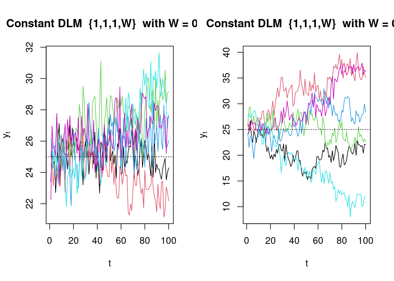
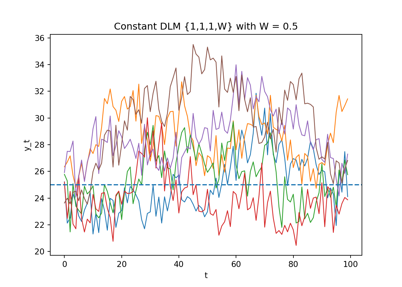
Write a computer program to graph 100 simulated observations from the DLM $\{1, 1, 1, W \}$ starting with $\mu_0 = 25$.
Simulate several series for each value of $W = 0.05$ and 0.5.
From these simulations, become familiar with the forms of behavior such series can display.
:::
::: {.solution}
Let's simulates/plots 100 observations from the constant DLM $\{F=1,G=1,V=1,W\}$ with $\mu_0=25$, for $W\in\{0.05,0.5\}$ Using R `DLM` library and the Python `pyDLM` package
:::: {.panel-tabset}
## R
```{r}
#| label: lst-sim-constant-dlm
#| echo: true
#| warning: false
# Simulate & plot constant DLM {1,1,1,W} with mu0=25 using dlm

library(dlm)

make_model <- function(W, m0 = 25, C0 = 0) {
  # Local-level DLM with V=1 and chosen W
  dlmModPoly(order = 1, dV = 1, dW = W, m0 = m0, C0 = C0)
}

sim_constant <- function(mod, n = 100, seed = NULL) {
  # Unconditional simulation from a 1D DLM
  if (!is.null(seed)) set.seed(seed)
  V <- as.numeric(mod$V); W <- as.numeric(mod$W)
  F <- as.numeric(mod$FF); G <- as.numeric(mod$GG)
  theta <- numeric(n); y <- numeric(n)
  th <- as.numeric(mod$m0)
  for (t in seq_len(n)) {
    th <- G * th + rnorm(1, 0, sqrt(W))   # state
    y[t] <- F * th + rnorm(1, 0, sqrt(V)) # observation
    theta[t] <- th
  }
  list(y = y, theta = theta)
}

simulate_replicates <- function(W, n = 100, R = 6, seed = 1) {
  mod <- make_model(W)
  lapply(seq_len(R), function(r) sim_constant(mod, n, seed + r))
}

plot_replicates <- function(sims, W) {
  Y <- do.call(cbind, lapply(sims, `[[`, "y"))
  matplot(Y, type = "l", lty = 1, lwd = 1,
          xlab = "t", ylab = expression(y[t]),
          main = paste0("Constant DLM  {1,1,1,W}  with W = ", W))
  abline(h = 25, lty = 3)
}

# --- run ---
par(mfrow = c(1, 2))
plot_replicates(simulate_replicates(W = 0.05, R = 6, seed = 42), W = 0.05)
plot_replicates(simulate_replicates(W = 0.5,  R = 6, seed = 4242), W = 0.5)
par(mfrow = c(1, 1))
```
## Python
```{python}
#| label: lst-sim-constant-dlm-py
# Simulate and plot constant DLM {F=1, G=1, V=1, W} with mu0=25
# Falls back to a pure NumPy simulator so it runs anywhere.
# If pyDLM is installed, you can later fit the same series with:
#   from pydlm import dlm, trend; dlm(y) + trend(1)
#
# Two figures are produced (no subplots): one for W=0.05 and one for W=0.5.

import numpy as np
import matplotlib.pyplot as plt

def simulate_constant_dlm(n: int, W: float, mu0: float = 25.0, V: float = 1.0, seed: int | None = None):
    """
    Simulate y_t from the constant DLM {F=1, G=1, V, W} with initial state theta_0 = mu0.
    State eq.:    theta_t = theta_{t-1} + omega_t,  omega_t ~ N(0, W)
    Obs eq.:      y_t     = theta_t + epsilon_t,    epsilon_t ~ N(0, V)
    Returns (y, theta).
    """
    rng = np.random.default_rng(seed)
    theta = np.empty(n, dtype=float)
    y = np.empty(n, dtype=float)
    th = mu0
    for t in range(n):
        th = th + rng.normal(0.0, np.sqrt(W))     # evolve
        y[t] = th + rng.normal(0.0, np.sqrt(V))   # observe
        theta[t] = th
    return y, theta

def simulate_replicates(W: float, n: int = 100, R: int = 6, seed: int = 0):
    """
    Generate R replicate series for given W. Seeds are offset to vary paths.
    Returns list of dicts with 'y' and 'theta'.
    """
    reps = []
    for r in range(R):
        y, th = simulate_constant_dlm(n=n, W=W, seed=seed + r)
        reps.append({"y": y, "theta": th})
    return reps

def plot_replicates(reps, W: float, mu0: float = 25.0, fname: str | None = None):
    """
    Plot multiple simulated observation series y_t for a fixed W.
    Saves figure if fname is provided.
    """
    plt.figure()
    for rep in reps:
        plt.plot(rep["y"], linewidth=1)
    plt.axhline(mu0, linestyle="--")
    plt.xlabel("t")
    plt.ylabel("y_t")
    plt.title(f"Constant DLM {{1,1,1,W}} with W = {W}")
    if fname:
        plt.savefig(fname, bbox_inches="tight", dpi=150)

# --- Run simulations and plotting ---
W_values = [0.05, 0.5]
paths = []
for W in W_values:
    reps = simulate_replicates(W=W, n=100, R=6, seed=42 if W == 0.05 else 4242)
    fname = f"constant_dlm_W{str(W).replace('.', '')}.png"
    plot_replicates(reps, W=W, fname=fname)
    paths.append(fname)

paths
```
::::
:::
::: {.callout-note}
### Comments {.unlisted .unnumbered}
* $W=0.05$: series stay close to 25 with mild wandering.
* $W=0.5$: visibly rougher random-walk level, larger meanders.
- TODO: To vary $V$ or $\mu_0$, they should be promoted to args in `simulate_replicates()` and `make_model()`.
- TODO: add margins to figures.
:::
::: {#exr-ch2-ex2}
### Posterior Updating as a Weighted Average
For the DLM $\{1, 1, V_t , W_t \}$ show that:
(a) the *posterior precision* of $(\mu_t \mid \mathcal{D}_t)$ is the sum of the *prior precision* of $(\mu_t \mid \mathcal{D}_{t-1})$ and the *observation precision* of $(Y_t \mid \mu_t)$, namely
$$
C_{t}^{-1} = R_{t}^{-1} + V_{t}^{-1}
$$
(b) the posterior mean of $(\mu_t \mid \mathcal{D}_t)$ is *a weighted average* of the sum of the prior mean $\mathbb{E}[\mu_t \mid \mathcal{D}_{t-1}]$ and the observation $Y_t$ with weights proportional to the precisions $R_{t}^{-1}$ and $V_{t}^{-1}$, namely
$$
m_t = C_t \left( R_{t}^{-1} m_{t-1} + V_{t}^{-1} Y_t \right)
$$
:::
::: {#exr-ch2-ex3}
### Recurrence Relations for Priors
Consider the DLM $\{1, 1, V_t , W_t\}$ extended so that $\nu_t \sim \mathcal{N}[\bar{v}_t , V_t]$ and $\omega_t \sim \mathcal{N}[\bar{w}_t , W_t]$ may have non-zero means.
Obtain the recurrence relations for $\{m_t , C_t\}$
(a) using Bayes' theorem
(b) deriving the joint distribution $(\mu_t , Y_t \mid \mathcal{D}_{t-1})$ and using normal theory to obtain the appropriate conditional distribution.
:::
::: {.solution .column-screen-inset-right }
### Introduction and assumption {.unnumbered}
As best as I cam tell this question extends [@west2013bayesian sec. 2.2]
We start by postulating the following model:
$$
\begin{aligned}
\mu_t&=\mu_{t-1}+\omega_t, & \cancel{\omega_t\sim\mathcal{N}(0,W_t)}\; & \omega_t\sim\mathcal N(\bar w_t,W_t), && \text{(sys.)}\\
Y_t&=\mu_t+\nu_t, & \cancel{ \nu_t\sim\mathcal{N}(0,V_t)}\; & \nu_t\sim\mathcal N(\bar v_t,V_t), && \text{(obs.)}\\
\mu_{t-1}\mid\mathcal D_{t-1} &\sim \mathcal{N}(m_{t-1},C_{t-1})
\end{aligned}
$$
### Recurrences {.unnumbered}
$$
\begin{aligned}
\textcolor{ForestGreen}{a_t} &= m_{t-1} + \textcolor{OliveGreen}{\bar w_t}
& \text{state prior mean (sys. drift)}\\
\textcolor{RoyalBlue}{R_t} &= C_{t-1} + \textcolor{CornflowerBlue}{W_t}
& \text{state prior var (sys. noise)}\\
\textcolor{Magenta}{f_t} &= \textcolor{ForestGreen}{a_t} + \textcolor{Fuchsia}{\bar v_t}
& \text{1-step forecast mean (obs. bias)}\\
\textcolor{Turquoise}{Q_t} &= \textcolor{RoyalBlue}{R_t} + \textcolor{Cyan}{V_t}
& \text{1-step forecast var (obs. noise)}\\
\textcolor{BrickRed}{A_t} &= \dfrac{\textcolor{RoyalBlue}{R_t}}{\textcolor{Turquoise}{Q_t}}
& \text{prior/forecast var (Kalman gain)}\\
\textcolor{Orange}{e_t} &= y_t - \textcolor{Magenta}{f_t}
& \text{forecast error (innovation)}\\[4pt]
\textcolor{Violet}{m_t} &= \textcolor{ForestGreen}{a_t} + \textcolor{BrickRed}{A_t}\,\textcolor{Orange}{e_t}
& \text{update (post. mean)}\\
\textcolor{Gray}{C_t} &= \textcolor{RoyalBlue}{R_t} - \textcolor{BrickRed}{A_t}\,\textcolor{RoyalBlue}{R_t}
= \textcolor{RoyalBlue}{R_t} - \dfrac{\textcolor{RoyalBlue}{R_t}^2}{\textcolor{Turquoise}{Q_t}}
& \text{update (post. var)}
\end{aligned}
$$
### Bayes step {.unnumbered}
$$
\begin{aligned}
\underbrace{p(\mu_t \mid \mathcal D_{t-1})}_{\text{prior}}
&= \mathcal N\!\big(\mu_t;\ \textcolor{ForestGreen}{a_t},\ \textcolor{RoyalBlue}{R_t}\big)\\
\underbrace{p(y_t \mid \mu_t,\mathcal D_{t-1})}_{\text{likelihood}}
&= \mathcal N\!\big(y_t;\ \mu_t+\textcolor{Fuchsia}{\bar v_t},\ \textcolor{Cyan}{V_t}\big)\\[6pt]
\log p(\mu_t\mid y_t,\mathcal D_{t-1})
&= -\tfrac12\!\left[
\underbrace{\dfrac{\big(\mu_t-\textcolor{ForestGreen}{a_t}\big)^2}{\textcolor{RoyalBlue}{R_t}}}_{\text{prior quadratic}}
+
\underbrace{\dfrac{\big(y_t-\textcolor{Fuchsia}{\bar v_t}-\mu_t\big)^2}{\textcolor{Cyan}{V_t}}}_{\text{likelihood quadratic}}
\right]+c
& \text{plug in Normal forms}\\[8pt]
&= -\tfrac12\!\left[
\Big(\tfrac1{\textcolor{RoyalBlue}{R_t}}+\tfrac1{\textcolor{Cyan}{V_t}}\Big)\mu_t^2
-2\mu_t\!\Big(\tfrac{\textcolor{ForestGreen}{a_t}}{\textcolor{RoyalBlue}{R_t}}
+\tfrac{y_t-\textcolor{Fuchsia}{\bar v_t}}{\textcolor{Cyan}{V_t}}\Big)
\right]+c'
& \text{collect terms}\\[8pt]
&= -\tfrac12\,\dfrac{\big(\mu_t-\textcolor{Violet}{m_t}\big)^2}{\textcolor{Gray}{C_t}}+c''
& \text{complete the square}
\end{aligned}
$$
with moments
$$
\boxed{
\begin{aligned}
\textcolor{Gray}{C_t}
&=\Big(\tfrac1{\textcolor{RoyalBlue}{R_t}}+\tfrac1{\textcolor{Cyan}{V_t}}\Big)^{-1}
=\textcolor{RoyalBlue}{R_t}-\dfrac{\textcolor{RoyalBlue}{R_t}^2}{\textcolor{Turquoise}{Q_t}},
& \text{posterior variance}\\[6pt]
\textcolor{Violet}{m_t}
&=\dfrac{\dfrac{\textcolor{ForestGreen}{a_t}}{\textcolor{RoyalBlue}{R_t}}
+\dfrac{y_t-\textcolor{Fuchsia}{\bar v_t}}{\textcolor{Cyan}{V_t}}}
{\dfrac1{\textcolor{RoyalBlue}{R_t}}+\dfrac1{\textcolor{Cyan}{V_t}}}
=\textcolor{ForestGreen}{a_t}
+\underbrace{\dfrac{\textcolor{RoyalBlue}{R_t}}{\textcolor{Turquoise}{Q_t}}}_{\textcolor{BrickRed}{A_t}\ \text{(Kalman gain)}}
\big(y_t-\textcolor{Fuchsia}{\bar v_t}-\textcolor{ForestGreen}{a_t}\big)
=\textcolor{ForestGreen}{a_t}+\textcolor{BrickRed}{A_t}\,\textcolor{Orange}{e_t},
& \text{posterior mean}
\end{aligned}
}
$$
---
### (a) derivation via Bayes theorem
$$
\begin{aligned}
p(\mu_t\mid\mathcal D_{t-1})&=\mathcal N(a_t,R_t) & \text{state evolution mean/var} \\
p(y_t\mid \mu_t)&=\mathcal N(\mu_t+\bar v_t,V_t) & \text{likelihood} \\
\Rightarrow\ \ \log p(\mu_t\mid y_t,\mathcal D_{t-1})
&= -\tfrac12\!\left[\frac{(\mu_t-a_t)^2}{R_t}+\frac{(y_t-\bar v_t-\mu_t)^2}{V_t}\right]+c & \text{Bayes, drop const} \\
&= -\tfrac12\!\left[(\tfrac1{R_t}+\tfrac1{V_t})\mu_t^2
-2\mu_t\!\left(\tfrac{a_t}{R_t}+\tfrac{y_t-\bar v_t}{V_t}\right)\right]+c' & \text{expand} \\
&= -\tfrac12\!\left[\frac{(\mu_t-m_t)^2}{C_t}\right]+c'' & \text{complete the square}
\end{aligned}
$$
$$
\begin{aligned}
&\underbrace{p(\mu_t \mid \mathcal D_{t-1})}_{\text{prior}}
=\mathcal N(\mu_t;\ a_t,R_t),
&& a_t=m_{t-1}+\bar w_t,\;\ R_t=C_{t-1}+W_t \\[4pt]
&\underbrace{p(y_t\mid \mu_t,\mathcal D_{t-1})}_{\text{likelihood}}
=\mathcal N(y_t;\ \mu_t+\bar v_t,V_t) \\[8pt]
p(\mu_t\mid y_t,\mathcal D_{t-1})
&\propto
\underbrace{p(y_t\mid \mu_t,\mathcal D_{t-1})}_{\text{likelihood}}\;
\underbrace{p(\mu_t \mid \mathcal D_{t-1})}_{\text{prior}}
& \text{Bayes}\\[4pt]
&\propto
\underbrace{\exp\!\Big[-\tfrac{(y_t-\bar v_t-\mu_t)^2}{2V_t}\Big]}_{\text{likelihood}}
\underbrace{\exp\!\Big[-\tfrac{(\mu_t-a_t)^2}{2R_t}\Big]}_{\text{prior}} \\[6pt]
&\propto
\exp\!\left\{-\tfrac12\!\left[
\underbrace{\tfrac{(\mu_t-a_t)^2}{R_t}}_{\text{prior quad.}}
+
\underbrace{\tfrac{(y_t-\bar v_t-\mu_t)^2}{V_t}}_{\text{likelihood quad.}}
\right]\right\}
& \text{collect terms}\\[6pt]
&=
\exp\!\left[-\tfrac12\,\tfrac{(\mu_t-m_t)^2}{C_t}\right],
\quad
\begin{cases}
\displaystyle C_t=\Big(\tfrac1{R_t}+\tfrac1{V_t}\Big)^{-1},\\[6pt]
\displaystyle m_t=\dfrac{\frac{a_t}{R_t}+\frac{y_t-\bar v_t}{V_t}}
{\frac1{R_t}+\frac1{V_t}}
= a_t+\dfrac{R_t}{R_t+V_t}\big(y_t-\bar v_t-a_t\big).
\end{cases}
& \text{complete square}
\end{aligned}
$$
with
$$
\boxed{
\begin{aligned}
m_t&=\frac{\frac{a_t}{R_t}+\frac{y_t-\bar v_t}{V_t}}{\frac1{R_t}+\frac1{V_t}}
= a_t + \frac{R_t}{R_t+V_t}\,\big(y_t-\bar v_t-a_t\big)
= a_t + A_t e_t,\\[3pt]
C_t&=\left(\frac1{R_t}+\frac1{V_t}\right)^{-1}
= \frac{R_t V_t}{R_t+V_t}
= R_t - \frac{R_t^2}{R_t+V_t}.
\end{aligned}}
$$
---
### (b) Via the joint normal and conditioning {.unnumbered}
$$
\begin{aligned}
\begin{bmatrix}\mu_t\\Y_t\end{bmatrix}\Bigm|\mathcal D_{t-1}
&\sim \mathcal N\!\left(
\begin{bmatrix}a_t\\ a_t+\bar v_t\end{bmatrix},
\begin{bmatrix}
R_t & R_t\\
R_t & R_t+V_t
\end{bmatrix}\right) & \text{sum of independent normals} \\
\Rightarrow\ \ \mu_t\mid Y_t=y_t,\mathcal D_{t-1}
&\sim \mathcal N\!\left(
a_t+\frac{R_t}{R_t+V_t}(y_t-a_t-\bar v_t),\ \ R_t-\frac{R_t^2}{R_t+V_t}
\right) & \text{BVN conditioning}
\end{aligned}
$$
which is the same $(m_t,C_t)$ as in (a).
---
### Summary (recurrences) {.unnumbered}
$$
\boxed{
\begin{aligned}
\text{Prior (evolution):}\quad & a_t=m_{t-1}+\bar w_t,\quad R_t=C_{t-1}+W_t.\\
\text{Forecast:}\quad & f_t=a_t+\bar v_t,\quad Q_t=R_t+V_t.\\
\text{Update:}\quad & A_t=\frac{R_t}{Q_t},\ \ e_t=y_t-f_t,\\
& m_t=a_t+A_t e_t,\quad C_t=R_t-A_t R_t=R_t-\frac{R_t^2}{Q_t}.
\end{aligned}}
$$
- The shocks just shift means;
- The Kalman‐style recursions are unchanged except the prediction/forecast means include $\bar{w}_t,\bar{v}_t$.
Only the means shift: $\bar w_t$ enters the prior mean, $\bar v_t$ enters the forecast mean; gains/variances are unchanged from the zero-mean case.
*Refs*: West & Harrison (1997, §4.3); Prado, Ferreira & West (2023, Ch. 1–2).
:::
::: {#exr-ch2-ex4-static-dlm}
### Static DLM
Show that the static DLM $\{1, 1, V, 0\}$, is equivalent to the model
$$
(Y_t \mid \mu) \sim \mathcal{N}[\mu, V], \quad (\mu \mid \mathcal{D}_0) \sim \mathcal{N}[m_0, C_0].
$$
Now suppose that $C_0$ is very large relative to $V$, so that $V C_0^{-1} \approx 0$.
Show that
(a)
$$
m_1 \approx Y_1
$$
and
$$
C_1 \approx V
$$
and
(b)
$$
m_t \approx \frac{1}{t} \sum_{j=1}^{t} Y_j
$$
and
$$
C_t \approx \frac{V}{t}.
$$
Comment on these results in relation to classical estimates.
:::
::: {#exr-ch2-ex5-constant-dlm}
### Constant DLM
For the constant DLM $\{1, 1, 100, 4\}$, if $(\mu_t \mid \mathcal{D}_t) \sim \mathcal{N}[200, 20]$, what are your forecasts of:
(a) $(Y_{t+4} \mid \mathcal{D}_t)$,
(b) $(Y_{t+1} + Y_{t+2} \mid \mathcal{D}_t)$,
(c) $(Y_{t+3} + Y_{t+4} \mid \mathcal{D}_t)$?
:::
::: {#exr-ch2-ex6-missing-observation}
### Missing Observation
Suppose that $Y_t$ is a missing observation, so that $\mathcal{D}_t = \mathcal{D}_{t-1}$. Given $(\mu_{t-1} \mid \mathcal{D}_{t-1}) \sim \mathcal{N}[m_{t-1}, C_{t-1}]$, obtain the distributions of $(\mu_t \mid \mathcal{D}_t)$ and $(Y_{t+1} \mid \mathcal{D}_t)$.
Do this for the constant DLM $\{1, 1, 100, 4\}$ when
$$
(\mu_{t-1} \mid \mathcal{D}_{t-1}) \sim \mathcal{N}[200, 40]
$$
:::
::: {#exr-ch2-ex7}
### Coping with Outliers
Bearing in mind the previous question, suggest a method for coping with outliers and general maverick observations with respect to subsequent forecasts.
:::
::: {#exr-ch2-ex8}
### Constant DLM with known changing observational and system variances.
For the DLM $\{1, 1, V_t, W_t\}$, with $(\mu_t \mid \mathcal{D}_{t-1}) \sim \mathcal{N}[m_{t-1}, R_t]$,
(a) obtain the joint distribution of $(\nu_t, Y_t \mid \mathcal{D}_{t-1})$.
(b) Hence prove that the posterior distribution for $\nu_t$ is
$$
(\nu_t \mid \mathcal{D}_t) \sim \mathcal{N}[(1 - A_t) e_t, A_t V_t].
$$
(c) Could you have deduced (b) immediately from $(\mu_t \mid \mathcal{D}_t)$?
:::
::: {#exr-ch2-ex9}
### Retrospective Analysis
It is often of interest to perform a *retrospective analysis* [**retrospective analysis**]{.column-margin} that looks back in time to make inferences about historical levels of a time
series based on all the current data.
As a simple case, consider inferences about $\mu_{t-1}$ based on $\mathcal{D}_t = \{ Y_t , \mathcal{D}_{t-1} \}$.
(a) Obtain the joint distribution $(\mu_{t-1} , Y_t \mid \mathcal{D}_{t-1})$;
(b) hence with $B_{t-1} = C_{t-1} / R_t$ deduce that
$(\mu_{t-1} \mid \mathcal{D}_t) \sim \mathcal{N}[a_t(-1), R_t(-1)]$,
where
$$
a_t(-1) = m_{t-1} + B_{t-1} (m_t - m_{t-1})
$$
and
$$
R_t(-1) = C_{t-1} - B_{t-1}^2 (R_t - C_t).
$$
(c) Write these equations for the discount DLM of [@west2013bayesian Section 2.4.2.]
:::
::: {#exr-ch2-ex10}
### Missing Observation
For the constant DLM $\{1, 1, V, W\}$, $(\mu_{t-1} \mid \mathcal{D}_{t-1}) \sim \mathcal{N}[m_{t-1}, C_{t-1}]$,
suppose that the data recording procedure at times $t$ and $t+1$ is such
that $Y_t$ and $Y_{t+1}$ cannot be separately observed, but $X = Y_t + Y_{t+1}$
is observed at $t + 1$. Hence $\mathcal{D}_t = \mathcal{D}_{t-1}$ and $\mathcal{D}_{t+1} = \{\mathcal{D}_{t-1}, X\}$.
(a) Obtain the distributions of $(X \mid \mathcal{D}_{t-1})$ and $(\mu_{t+1} \mid \mathcal{D}_{t+1})$.
(b) Generalize this result to the case
$$
X = \sum_{v=0}^{k} Y_{t+v} \text{ and } \mathcal{D}_{t+k} = \{X, \mathcal{D}_{t-1}\}
$$
(c) For integers $j$ and $k$ such that $0 \le j < j + k$, find the forecast
distribution of
$$
\sum_{v=j}^{j+k} Y_{t+v} \text{ given } \mathcal{D}_{t-1}
$$
:::
::: {#exr-ch2-ex11}
### Coping with Uncertainty
There is a maxim,
> “When in doubt about a parameter value, err on the side of more uncertainty.”
To investigate this, repeat the exercise of Example 2.1 using in turn the following prior settings:
(a) $(\mu_0 \mid \mathcal{D}_0) \sim \mathcal{N}[650, 100000]$
(b) $(\mu_0 \mid \mathcal{D}_0) \sim \mathcal{N}[130, 4]$
(c) $(\mu_0 \mid \mathcal{D}_0) \sim \mathcal{N}[11, 1]$
In particular, examine the time graphs of $\{A_t\}$, $\{f_t, f_t \pm Q_t, Y_t\}$,
and of $\{m_t, Y_t\}$.
What conclusions do you draw?
We once designed a more general forecasting system which the customer tried to break by setting priors with silly prior means $m_0$ and large variances $C_0$.
He drew the conclusion that the system was so robust it could not be broken.
How would you show that it could be broken if it were not protected by a monitoring system?
:::
::: {#exr-ch2-ex12}
### Discount Factors high and low
Another maxim is,
> "In a complete forecast system higher rather than lower values of the discount factor are to be preferred."
Investigate this by redoing Example 2.1 using the prior $(\mu_0 \mid \mathcal{D}_0) \sim \mathcal{N}[130, 400]$ but employing the discount DLM so that $R_t = C_{t-1} / \delta$. Use in turn the discount factors $\delta = 0.8, 1.0$ and $0.01$. In particular, examine time graphs of the $\{f_t , C_t \}$ in each case.
- What conclusions do you draw?
- Do you see any mimicry?
- Too many systems fall between two stools in trying to select adaptive/discount factors that will not overly respond to random fluctuations yet will quickly adapt to major changes; the result is an unsatisfactory compromise.
A complete forecasting system generally chooses high discount factors, usually $0.8 \leq \delta < 0.99$, to capture the routine system movements but relies on a monitoring system to signal major changes that need to be brought to the notice of decision makers and that require expert intervention.
:::
::: {#exr-ch2-ex13}
### Limiting Identities in Constant DLM
In the constant DLM $\{1, 1, V, W\}$, verify the limiting identities
$$
R = \frac{A V}{1 - A}, \qquad
Q = \frac{V}{1 - A}, \qquad
W = A^2 Q.
$$
:::
::: {#exr-ch2-ex14}
### Closed Constant DLM
In the closed, constant DLM with limiting values $A$, $C$, $R$, etc., prove that the sequence $C_t$ decreases/increases as $t$ increases according to whether $C_0$ is greater/less than the limiting value $C$. Show that the sequence $A_t$ behaves similarly.
:::
::: {#exr-ch2-ex15}
### Discount Weighted Regression (DWR)
Discount weighted regression applied to a locally constant process estimates the current level at time $t$ as that value $M_t$ of $\mu$ that, given $Y_1, \ldots, Y_t$, minimises the discounted sum of squares
$$
S_t(\mu) = \sum_{j=0}^{t-1} \delta^j \left( Y_{t-j} - \mu \right)^2 .
$$
(a) Prove that $M_t$ is a discount weighted average of the $t$ observations
$$
M_t = \frac{1 - \delta}{1 - \delta^t} \sum_{v=0}^{t-1} \delta^v Y_{t-v} .
$$
(b) Show that writing $e_t = Y_t - M_{t-1}$, neat recurrence forms are
$$
M_t = \frac{1 - \delta}{1 - \delta^{t}} Y_t + \frac{\delta(1 - \delta^{t-1})}{1 - \delta^t} M_{t-1}
$$
and
$$
M_t = M_{t-1} + \frac{1 - \delta}{1 - \delta^t} e_t .
$$
(c) Show that as $t \to \infty$ the limiting form of this recurrence relationship is that of Brown’s method of EWR, Section 2.3.5(c),
$$
M_t = \delta M_{t-1} + (1 - \delta) Y_t = M_{t-1} + (1 - \delta) e_t .
$$
:::
::: {#exr-ch2-ex16}
### DWR and the Constant DLM
In the context of question (16) on DWR, note that as $t \to \infty$,
$$
V[e_t \mid \mathcal{D}_{t-1}] \to Q \text{ and } (Y_{t+1} - Y_t - e_{t+1} + \delta e_t) \to 0
$$
This suggests that the process can be modelled as
$$
Y_{t+1} - Y_t = a_{t+1} - \delta a_t,
$$
where $a_t \sim \mathcal{N}[0, Q]$ are independent random variables.
Then an estimate of $Q$ given $Y_{t+1}, \ldots, Y_1$ is
$$
\hat{Q}(t + 1) = \frac{1}{t} \sum_{v=1}^t \frac{ (Y_{v+1} - Y_v)^2}{1 + \delta^2}.
$$
(a) Do you consider this a reasonable point estimate of $Q$?
(b) Show that
$$
\hat{Q}(t + 1) = \hat{Q}(t) + \frac{1}{t} \left[ \frac{(y_{t+1} - y_t)^2 }{1 + \delta^2} - \hat{Q}(t) \right]
$$
and that a reasonable point estimate of $V[Y_t \mid \mathcal{D}_{t-1}]$ is
$$
\hat{Q}_t = \left\{ \delta + \frac{(1 - \delta)(1 - \delta^t)}{(1 - \delta^{t-1})^2} \right \} \, \hat{Q}(t - 1)
$$
with $t - 1$ degrees of freedom.
:::
::: {#exr-ch2-ex17}
### Discount DLM with Constant Discount Factor
In the $\{1, 1, V, W_t\}$ discount DLM with constant discount factor $\delta$,
suppose that $C_0$ is very large relative to $V$. Show that
(a)
$$
C_t \approx \frac{V (1 - \delta)}{1 - \delta^t}, \qquad \forall t \ge 1
$$
(b)
$$
m_t \approx \frac{1 - \delta}{1 - \delta^t} \sum_{j=0}^{t-1} \delta^j Y_{t-j},
$$
(c)
$$
m_t \approx \frac{1 - \delta}{1 - \delta^t} Y_t +
\frac{1 - \delta^{t-1}}{1 - \delta^t} \, \delta \, m_{t-1},
$$
(d)
$$
m_t \approx m_{t-1} + \frac{1 - \delta}{1 - \delta^t} \, e_t.
$$
(e) Compare these results with those of the relevant DWR approach in question (16) above.
What do you conclude? What do you think about applying that variance estimate $\hat{Q}_t$ of $Q$, from question (16), to this DLM?
If you do adopt the method, what is the corresponding point estimate of $V$?
:::
::: {#exr-ch2-ex18}
### Constant DLM Updating Equations
In the constant DLM $\{1, 1, V, W\}$, show that $R_t = C_{t-1}/\delta_t$, where $\delta_t \in (0,1]$. Thus, the constant DLM updating equations are equivalent to those in a discount DLM with discount factors $\delta_t$ changing over time. Find the limiting value of $\delta_t$ as $t$ increases, and verify that $\delta_t$ increases/decreases with $t$ according to whether the initial variance $C_0$ lies below/above the limiting value $C$.
:::
::: {#exr-ch2-ex19}
### Lead Time Forecast Variance
Consider the lead time forecast variance $L_t(k)$ in Section 2.3.6.
(a) Show that the value of $k$ minimizing the lead time coefficient of
variation is independent of $C_t$. What is this value when $V = 97$
and $W = 6$?
(b) Supposing that $C_t = C$, the limiting value, show that the
corresponding value of $L_t(k)/V$ depends only on $k$ and $r = W/V$.
For each value of $r = 0.05$ and $r = 0.2$, plot the ratio $L_t(k)/V$
as a function of $k$ over $k = 1, \ldots, 20$.
Comment on the form of the plots and the differences between the two cases.
:::
::: {#exr-ch2-ex20}
### Heavy-tailed Student t Distributions
Become familiar with just how heavy-tailed Student T distributions
with small and moderate degrees of freedom are relative to normal
distributions.
To do this graph the distribution using an appropriate computer package and find the upper 90%, 95%, 97.5% and 99%
points of the $\mathcal{T}_n[0, 1]$ distribution for n =2, 5, 10 and 20 degrees
of freedom, comparing these with those of the $\mathcal{N}[0, 1]$ distribution.
~~~Statistical tables can also be used (Lindley and Scott, 1984, p45).~~~
:::
::: {#exr-ch2-ex21}
### Sensitivity Analysis of the DLM for Exchange Rates
Perform analyses of the USA/UK exchange rate index series along the lines of those in Section 2.6, one for each value of the discount factor $\delta = 0.6, 0.65, \ldots, 0.95, 1$.
Relative to the DLM with $\delta = 1$, plot the *MSE*, *MAD* and *LLR* measures as functions of $\delta$.
Comment on these plots.
[**Sensitivity analysis**]{.column-margin} Sensitivity analyses explore how inferences change with respect to model assumptions. At $t = 115$, explore how sensitive this model is to values of $\delta$ in terms of inferences about the final level $\mu_{115}$, the variance $V$ and the next observation $Y_{116}$.
:::
::: {#exr-ch2-ex22}
### Autocorrelation in the DLM
In the DLM $\{1, 1, 1, W\}$, define $Z_t = Y_{t+1} - Y_t$.
Show that for integer $k$ such that $|k| > 1$,
$$
E[Z_t] = 0,\quad
V[Z_t] = 2 + W,\quad
C[Z_t, Z_{t-1}] = -1
$$
and $C[Z_t, Z_{t+k}] = 0$. Based upon $n + 1$ observations $(Y_1, \ldots, Y_{n+1})$,
giving the $n$ values $(Z_1, \ldots, Z_n)$, the usual sample estimate of the
autocorrelation coefficient of lag $k$, $C[Z_t, Z_{t+k}]/V[Z_t]$, is
$$
r_k = \frac{\sum_{i=1}^{n-k} Z_{i+k} Z_i}{\sum_{i=1}^{n} Z_i^2}.
$$
Using the computer program of question 1, generate 100 values of $z_i$
and plot the sample autocorrelation graph $\{r_k, k : k = 0, \ldots, 12\}$
for $W = 0.05$ and also $W = 0.5$.
Assuming the model true, the prior marginal distribution of $r_k$, for every $|k| > 1$, is roughly $\mathcal{N}[0, 1/\sqrt{n}]$.
Do the data support or contradict the model?
This is an approach used in identifying the constant DLM and an ARIMA(0,1,1) model.
Supposing the more general DLM $\{1, 1, V_t, W_t\}$, show that again
$C[Z_t, Z_{t+k}] = 0$ for all $|k| > 1$, so the graph $\{r_k, k : k > 1\}$
is expected to look exactly the same.
Note also that if $V_t/W_t$ is constant, the whole graph $\{r_k, k\}$ is expected to look exactly the same.
What is $r_k$ now measuring and what are the implications for identifying the constant DLM and the ARIMA(0,1,1)?
:::
::: {#exr-ch2-ex23}
Suppose an observation series $\{Y_t\}$ is generated by the constant DLM $\{1, 1, V^*, W^*\}$. We can write $Y_t - Y_{t-1} = a_t - \delta^* a_{t-1}$ where $a_t \sim \mathcal{N}[0, Q^*]$ are independent random variables and $Q^*$ is the associated limiting one-step forecast variance. In order to investigate robustness, suppose a non-optimal DLM $\{1, 1, V, W\}$ is employed, so that in the limit, $Y_t - Y_{t-1} = e_t - \delta e_{t-1}$ where the errors will have a larger variance $Q$ and no longer be independent. Show that for integer $k$ such that $\lvert k \rvert \ge 1$,
$$
Q = \mathbb{V}[e_t] = \left[1 + \frac{(\delta - \delta^*)^2}{1 - \delta^2}\right] Q^*
$$
and
$$
C(k) = \mathbb{C}[e_{t+k}, e_t] = \delta^{\lvert k \rvert - 1} \, Q^* \, \frac{(\delta - \delta^*)(1 - \delta \delta^*)}{1 - \delta^2}.
$$
Examine graphs of $\{\delta, Q/Q^*\}$ and of $\{\delta, C(1)/Q\}$ for the typical practical cases $\delta^* = 0.9, \delta^* = 0.8$ and for the atypical case $\delta^* = 0.5$.
:::