---
date: 2024-11-03
title: "The AR(1): MLE and Bayesian inference"
subtitle: Time Series Analysis
description: "This lesson we will define the AR(1) process, Stationarity, ACF, PACF, differencing, smoothing"
categories:
- bayesian statistics
keywords:
- notes
- time series
- autoregressive models
- stationarity
- MLE
- AR(1) process
- Yule-Walker equations
- Durbin-Levinson recursion
- Moore-Penrose pseudoinverse
- Full Rank Matrix
- R code
---
::: {.callout-note collapse="true"}
## Learning Objectives
- [x] Perform maximum likelihood estimation for the full and conditional likelihood in an AR(1) [\#](#l2g3)
- [x] Perform Bayesian inference for the **AR(1)** under the conditional likelihood and the reference prior [\#](#l2g4)
:::
## Maximum likelihood and Bayesian inference in regression :spiral_notepad: {#sec-mle-bayes-regression}
This section is based on the handout provided in the course materials.
The gist of this handout is that if we can write the regression as the equation of a straight line, we should be able to make use of basic algebra to invert the equation and obtain an expression for the regression coefficients. We do this by writing the equation in matrix form and then using the Moore-Penrose pseudoinverse to obtain the maximum likelihood estimator for the regression coefficients.
::: {.callout-caution}
### Moore-Penrose pseudoinverse {.unnumbered}
Prado snuck the Moore-Penrose pseudoinverse in this handout, then she used it in the class and notes. I thought this isn't the first time this has come up in the specialization as we used MLE to some degree in all the courses, and in depth in the previous course on mixtures. However a cursory review did not uncover previous use of this mathematical tool. So I thought it might be useful to provide a brief overview of the Moore-Penrose pseudoinverse, its properties and how it is used in regression models.
Moore-Penrose pseudoinverse is a generalization of the inverse matrix that can be applied to non-square matrices.
- It is not covered in typical linear algebra courses. It might come up in numerical methods courses or a second linear algebra course. But unless they cover application in regression models, it is quite likely that they skip an important point, that [the Moore-Penrose pseudoinverse is used to obtain the maximum likelihood estimator for the regression coefficients in linear regression models.]{.mark}
I found a couple of reference in [@schott2016matrix ch. 5] but they it didn't cover they MLE aspect of the pseudoinverse.
I cover some of this material in an @sec-moore-penrose to the course notes, however I am still missing a good source for @eq-mle-estimator-beta.
<!-- TODO: Find a good reference for the MLE estimator for beta in the context of the Moore-Penrose pseudoinverse. and add it to the the appendix above -->
It is denoted as $X^+$ and has the following properties:
This pseudo-inverse is a neat bit of mathematics which allows us to not only invert the equation from the left but it somehow minimizes the sum of squared errors in the regression - I.e. we get the parameters while minimizing the sum of squared errors due to the variance term. One strong assumption we must make is that the design matrix $X$ is full rank, which means that the columns of the matrix are linearly independent. The columns of the design matrix correspond to the explanatory variables in the regression model.
In reality as we are dealing with hierarchical models, so we will not always have a full rank design matrix, but we can still use the Moore-Penrose pseudoinverse to obtain the maximum likelihood estimator for the regression coefficients.
:::
### Regression Models: Maximum Likelihood Estimation
\index{regression!linear}
\index{Maximum Likelihood Estimation}
Assume a regression model with the following structure:
$$
y_i = \beta_1x_{i,1} + \ldots + \beta_kx_{i,k} + \varepsilon_i,
$$
for $i = 1, \ldots, n$ and $\varepsilon_i$ independent random variables with $\varepsilon_i \sim \mathcal{N}(0, v) \quad \forall i$.
This model can be written in matrix form as:
$$
y = \mathbf{X} \boldsymbol{\beta} + \boldsymbol\varepsilon \qquad \boldsymbol\varepsilon \sim \mathcal{N} (0, v\mathbf{I})
$$
where:
- $y = (y_1, \ldots, y_n)′$ is an n-dimensional vector of responses,
- $\mathbf{X}$ is an $n × k$ matrix containing the explanatory variables,
- $\boldsymbol \beta = (\beta_1, \ldots, \beta_k)'$ is the k-dimensional vector of regression coefficients,
- $\boldsymbol \varepsilon = (\varepsilon_1, \ldots, \varepsilon_n)'$ is the n-dimensional vector of errors,
- $\mathbf{I}$ is an $n \times n$ identity matrix.
If $\mathbf{X}$ is a *full rank* matrix with rank $k$ , the maximum likelihood estimator for $\boldsymbol\beta$, denoted as $\hat{\boldsymbol\beta}_{MLE}$ is given by:
$$
\hat{\boldsymbol{\beta}}_{MLE} = (\mathbf{X}'\mathbf{X})^{−1}\mathbf{X}'\mathbf{y},
$$ {#eq-mle-estimator-beta}
\index{Moore-Penrose pseudoinverse}
where $(X^+ = \mathbf{X}'\mathbf{X})^{−1}\mathbf{X}'$ is the [Moore-Penrose pseudoinverse](https://en.wikipedia.org/wiki/Moore%E2%80%93Penrose_inverse) of the matrix $\mathbf{X}$. This Moore-Penrose pseudoinverse of the matrix $\mathbf{X}$ is the most widely known generalization of the inverse matrix and is used to obtain the least squares solution to the linear regression problem.
and the MLE for $v$ is given by:
$$
\hat{v}_{MLE} = \frac{1}{n} (y − \mathbf{X} \hat{\boldsymbol{\beta}}_{MLE})′(y − \mathbf{X} \hat{\boldsymbol{\beta}}_{MLE})
$$ {#eq-mle-estimator-v}
$\hat{v}_{MLE}$ is not an unbiased estimator of $v$, therefore, the following unbiased estimator of $v$ is typically used:
$$
s^2 = \frac{1}{n-k}(y − \mathbf{X} \hat{\boldsymbol\beta}_{MLE} )′(y − \mathbf{X} \hat{\boldsymbol\beta}_{MLE} )
$$ {#eq-mle-unbiased-estimator-v}
### Regression Models: Bayesian Inference {#sec-bayes-regression}
Assume once again we have a model with the structure in (1), which results in a likelihood of the form
$$
\mathbb{P}r(y \mid \boldsymbol{\beta} , v) = \frac{1}{(2\pi v)^{n/2}}\exp \left\{ -\frac{1}{2} (y − \mathbf{X} \boldsymbol{\beta})′(y − \mathbf{X} \boldsymbol{\beta}) \right\}
$$
If a prior of the form :
$$
\mathbb{P}r(\boldsymbol{\beta}, v) \propto \frac{1}{v}
$$ {#eq-prior-regression}
is used, we obtain that the posterior distribution is given by:
$$
\mathbb{P}r(\boldsymbol{\beta},v \mid \mathbf{y}) \propto \frac{1}{v^{n/2+1}}\exp \left\{ -\frac{1}{2v} (\mathbf{y} − \mathbf{X} \boldsymbol{\beta})′(\mathbf{y} − \mathbf{X} \boldsymbol{\beta}) \right\}
$$ {#eq-posterior-regression}
In addition it can be shown that
- $(\boldsymbol{\beta}\mid v, \mathbf{y}) \sim \mathcal{N} (\hat{\boldsymbol{\beta}}_{MLE} , v(\mathbf{X}'\mathbf{X})^{-1})$
- $(v \mid \mathbf{y}) \sim \mathcal{IG}\left(\frac{(n − k)}{2}, \frac{1}{2}d\right)$ with
$$
d = (\mathbf{y} − \mathbf{X} \hat{\boldsymbol{\beta}}_{MLE} )′(\mathbf{y} − \mathbf{X} \hat{\boldsymbol{\beta}}_{MLE} )
$$ {#eq-d-unbiased-estimator-v}
where $\mathcal{IG}(a, b)$ denotes the inverse-gamma distribution with *shape* parameter $a$ and *scale* parameter $b$.
with $k = dim(\boldsymbol\beta)$.
[Given that $\mathbb{P}r(\boldsymbol\beta, v \mid \mathbf{y}) = \mathbb{P}r(\boldsymbol\beta \mid v, \mathbf{y})p(v \mid \mathbf{y})$ the equations above provide a way to directly sample from the posterior distribution of $\boldsymbol \beta$ and $v$ by first sampling v from the inverse-gamma distribution above and then conditioning on this sampled value of v, sampling $\boldsymbol \beta$ from the normal distribution above.]{.mark}
## Maximum likelihood estimation in the AR(1) :movie_camera: {#sec-mle-ar1}
{#fig-s_0041 .column-margin group="slides" width="53mm"}
{#fig-s_0042 .column-margin group="slides" width="53mm"}
{#fig-s_0043 .column-margin group="slides" width="53mm"}
There are two main strategies for performing MLE for an AR(1) model:
- Full Likelihood: Considers the joint distribution of all observations $y_1, \dots, y_T$.
- Conditional Likelihood: Conditions on the first observation ($y_1$) and works with the likelihood of the remaining observations ($y_2, \dots, y_T$).
### **Model Setup**
The focus is on the **zero-mean AR(1) model**:
$$
Y_t = \phi Y_{t-1} + \varepsilon_t, \quad \varepsilon_t \overset{iid}{\sim} \mathcal{N}(0, v), \quad \phi \in (-1,1)
$$
This condition ensures **stationarity** of the process.
### **Distributional Assumptions**
* $Y_1 \sim \mathcal{N}\left(0, \frac{v}{1 - \phi^2}\right)$
* $Y_t \mid Y_{t-1} \sim \mathcal{N}(\phi Y_{t-1}, v)$ for $t \geq 2$
### **Likelihood Approaches**
Two approaches are considered:
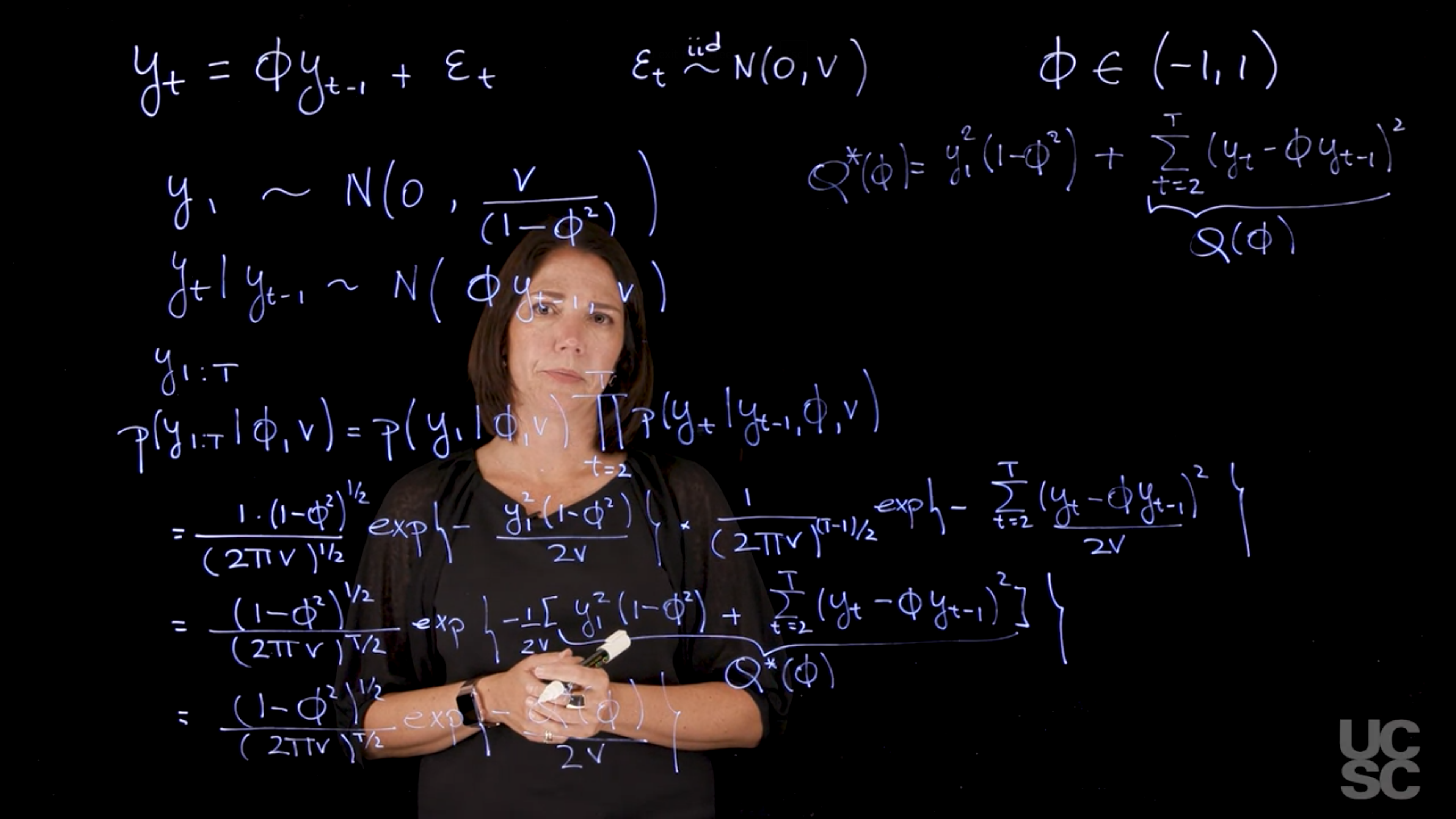
#### 1. **Full Likelihood**
$$
\begin{aligned}
p(y_{1:T} \mid \phi, v) &= p(y_1 \mid \phi, v) \cdot \prod_{t=2}^T p(y_t \mid y_{t-1}, \phi, v) \\
&= \frac{1}{\sqrt{2\pi \frac{v}{1 - \phi^2}}} \exp\left( -\frac{y_1^2 (1 - \phi^2)}{2v} \right) \cdot \prod_{t=2}^T \frac{1}{\sqrt{2\pi v}} \exp\left( -\frac{(y_t - \phi y_{t-1})^2}{2v} \right) \\
&= \frac{(1 - \phi^2)^{1/2}}{(2\pi v)^{T/2}} \cdot
\exp\left( -\frac{1}{2v} \left[ \underbrace{ y_1^2(1 - \phi^2) + \sum_{t=2}^T (y_t - \phi y_{t-1})^2 }_{\text{Quadratic Loss } Q^*(\phi)} \right] \right) \\
&= \frac{(1 - \phi^2)^{1/2}}{(2\pi v)^{T/2}} \exp\left( -\frac{Q^*(\phi)}{2v} \right)
\end{aligned}
$$ {#eq-full-likelihood-ar1}
where $Q^*(\phi)$ is defined as:
$$
Q^*(\phi) =
\underbrace{y_1^2(1 - \phi^2)\vphantom{\sum_{t=2}^T (y_t - \phi y_{t-1})^2}}_{\text{Initial Loss}}
+ \underbrace{\sum_{t=2}^T (y_t - \phi y_{t-1})^2}_{\text{Remaining Loss } Q(\phi)}
$$ {#eq-qstar-ar1}
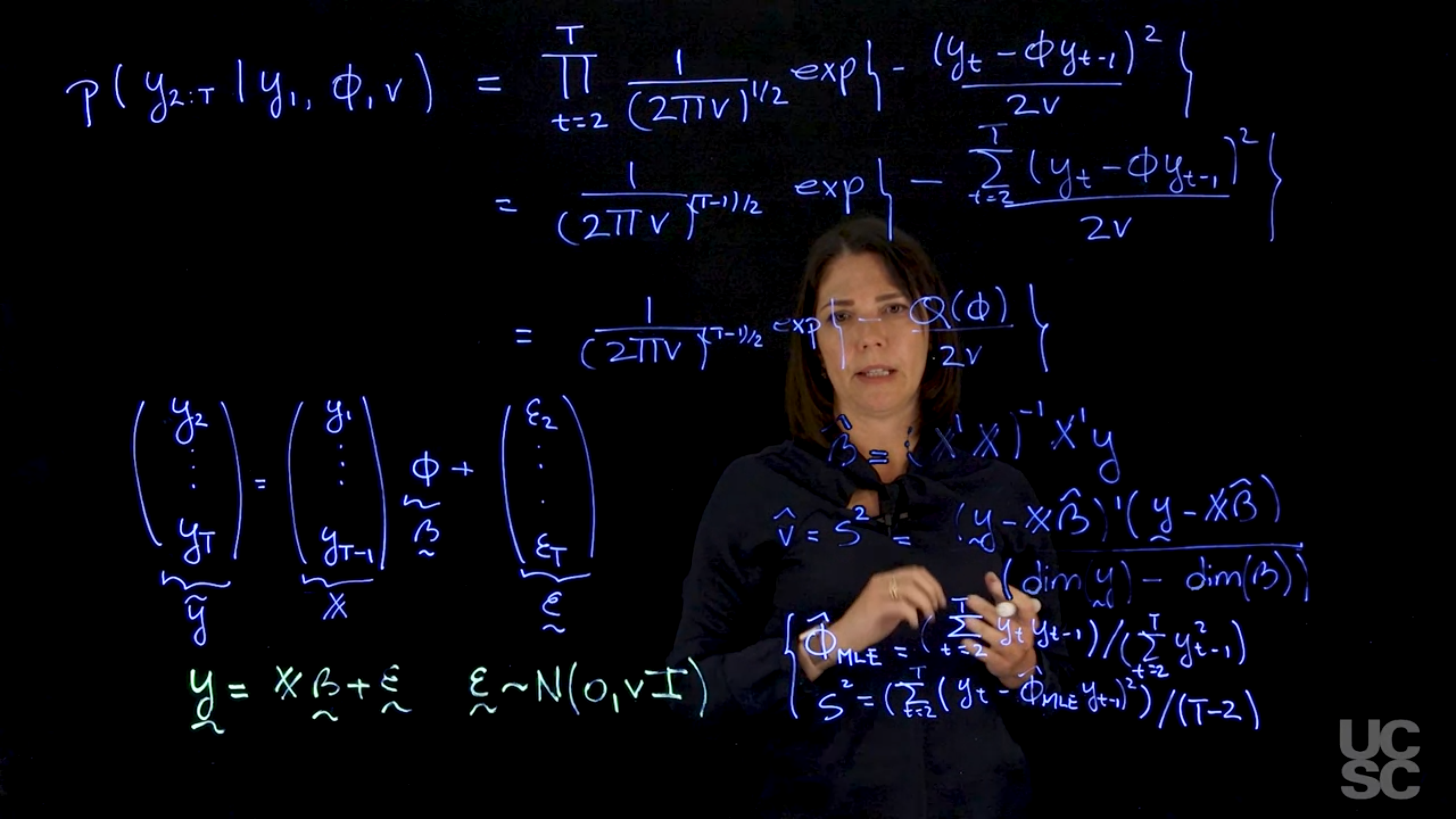
$$
\begin{aligned}
p(y_{1:T} \mid \phi) &= \prod_{t=2}^T \frac{1}{\sqrt{2\pi v}} \exp\left( -\frac{(y_t - \phi y_{t-1})^2}{2v} \right) \\
&= \frac{1}{(2\pi v)^{T/2}} \exp\left( -\sum_{t=2}^T \frac{1}{2v} \left( y_t - \phi y_{t-1} \right)^2 \right) \\
&= \frac{1}{(2\pi v)^{T/2}} \exp\left( -\frac{Q(\phi)}{2v} \right)
\end{aligned}
$$ {#eq-likelihood-ar1}
where $Q(\phi)$ is the quadratic loss function defined as:
$$
\underbrace{ \begin{pmatrix}y_1 \\ y_2 \\ \vdots \\ y_T \end{pmatrix} }_{\utilde{y}} =
\underbrace{ \begin{pmatrix}y_1 \\ y_2 \\ \vdots \\ y_T \end{pmatrix} }_{\mathbb{X}}
\underbrace{ \phi \vphantom{\begin{pmatrix}y_1 \\ y_2 \\ \vdots \\ y_T \end{pmatrix} }}_{\beta} +
\underbrace{ \begin{pmatrix}\varepsilon_1 \\ \varepsilon_2 \\ \vdots \\ \varepsilon_T\end{pmatrix}}_{\utilde {\varepsilon}}
$$ {#eq-ar1-model}
where $\utilde{y}$ is the vector of observations, $\mathbb{X}$ is the design matrix with $y_1$ as the first column and $y_2, \ldots, y_{T-1}$ as the second column, $\beta = \phi$ is the AR coefficient, and $\utilde{\varepsilon} \sim \mathcal{N}(0, vI)$ is the error term.
$$
\utilde{y} = \mathbb{X} \beta + \utilde{\varepsilon} \qquad \utilde{\varepsilon} \sim \mathcal{N}(0, vI)
$$
where $\mathbb{X}$ is the design matrix
with $y_1$ as the first column and $y_2, \ldots, y_{T-1}$ as the second column.
If the matrix $\mathbb{X}$ is full rank, the MLE for $\phi$ can be obtained as:
$$
\hat{\beta} = (\mathbb{X}'\mathbb{X})^{-1}\mathbb{X}'y
$$
and the MLE for $v$ is given by:
$$
\hat{v} = S^2 = \frac{(y - \mathbb{X}\hat{\beta})'(y - \mathbb{X}\hat{\beta})}{\dim(y)-\dim(\beta)}
$$
and the MLE for $\phi$.
$$
\hat{\phi}_{MLE} = \frac{\sum_{t=2}^T y_t y_{t-1}}{\sum_{t=2}^T y_{t-1}^2}
$$ {#eq-mle-ar1-phi}
and the unbiased estimator for $v$ is given by:
$$
S^2 = \sum_{t=2}^T (y_t - \hat{\phi}_{MLE} y_{t-1})^2 / (T - 2)
$$ {#eq-mle-ar1-v-unbiased}
where $T$ is the number of time points and $S^2$ is the unbiased estimator for the variance $v$.
And we usually use this unbiased estimator for $v$ in practice, as the MLE for $v$ is biased.
#### 2. **Conditional Likelihood**
Maximizing the full likelihood requires **numerical optimization methods** (e.g., Newton-Raphson), as there's no closed-form solution.
This setup is equivalent to a **linear regression**:
$$
\mathbf{y} = X\beta + \varepsilon, \quad \varepsilon \sim \mathcal{N}(0, vI)
$$
Where:
* $\mathbf{y} = [y_2, \dots, y_T]^T$
* $X = [y_1, \dots, y_{T-1}]^T$
* $\beta = \phi$
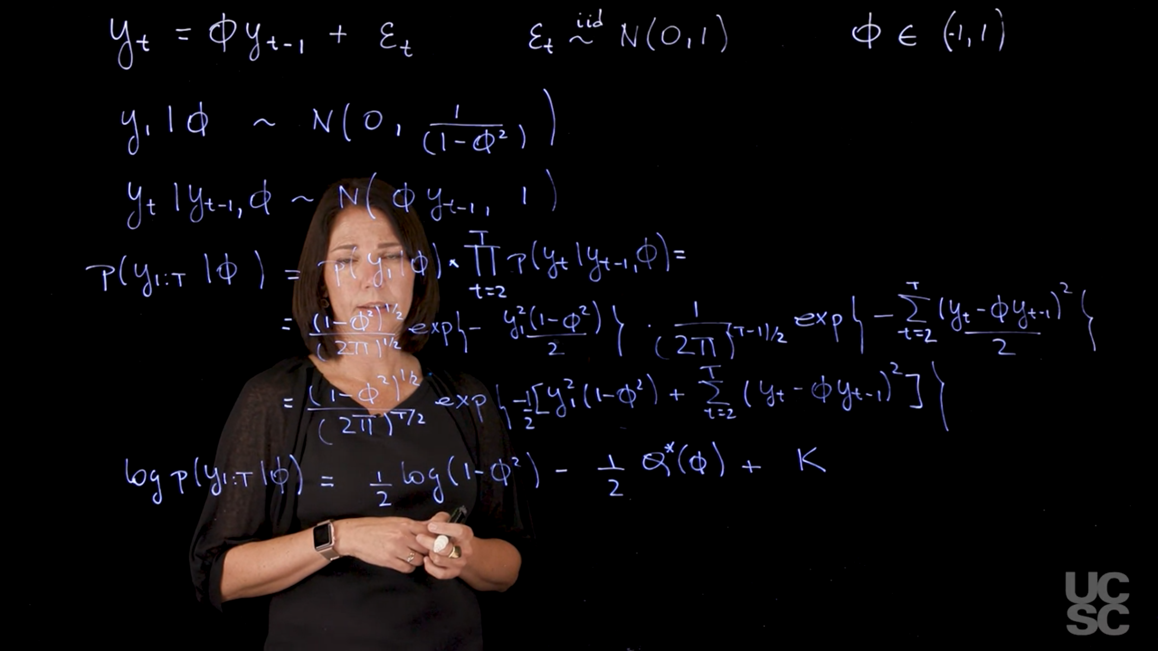
Condition on $y_1$:
$$
\begin{aligned}
p(y_1 \mid \phi) &\sim \mathcal{N}(0, 1/(1 - \phi^2)) \\
p(y_t \mid y_{t-1}, \phi) &\sim \mathcal{N}(\phi y_{t-1}, 1) \\
\end{aligned}
$$
$$
\begin{aligned}
p(y_{1:T} \mid y_1, \phi, v) &= p(y_1 \mid \phi) \cdot \prod_{t=2}^T p(y_t \mid y_{t-1}, \phi)\\
&= \frac{(1 - \phi^2)^{1/2}}{(2\pi)^{T/2}} \exp\left(-\frac{y_1^2(1 - \phi^2)}{2}\right) \cdot \prod_{t=2}^T \frac{1}{\sqrt{2\pi}} \exp\left(-\frac{(y_t - \phi y_{t-1})^2}{2}\right) \\
&= \frac{(1 - \phi^2)^{1/2}}{(2\pi)^{T/2}} \exp\left(-\frac{1}{2} \left[y_1^2(1 - \phi^2) + \sum_{t=2}^T (y_t - \phi y_{t-1})^2\right]\right) \\
\end{aligned}
$$
So the log-likelihood becomes:
$$
\log p(y_{1:T} \mid y_1, \phi) = \frac{1}{2} \log(1 - \phi^2) - \frac{1}{2} Q(\phi) + K
$$ {#eq-log-likelihood-ar1}
where $K$ is a constant that does not depend on $\phi$.
So if I were to look at maximizing this function, we can think about taking first derivatives with respect to phi. And then we will see that again the expression that you obtain doesn't allow you to obtain a close form expression for $\hat{\phi}_{MLE}$. Instead, we will need to use a numerical optimization method such as Newton Raphson to obtain the maximum likelihood estimator for phi.
### Conclusion
* **Full likelihood** is more general but computationally intensive.
* **Conditional likelihood** simplifies estimation by leveraging regression theory.
* When variance $v$ is known (e.g., $v = 1$), the optimization reduces to maximizing a univariate function of $\phi$.
* For full likelihood, optimization of $Q^*(\phi)$ is required.
| Feature | Full Likelihood | Conditional Likelihood (Regression) |
| --------------------- | --------------------------- | ------------------------------------------|
| Accounts for $Y\_1$ | ✅ Yes | ❌ No |
| MLE for $\phi$ | ❌ No closed form | ✅ Closed form |
| MLE for $v$ | ❌ Biased unless adjusted | ✅ Unbiased estimator available |
| Optimization Needed | ✅ Yes (numerical methods) | ❌ No (closed-form MLE for $\phi$) |
| Useful when | Modeling full joint process | Estimating $\phi$ efficiently in practice |
::: {.callout-note collapse="true"}
## Video Transcript
{{< include transcripts/c4/01_week-1-introduction-to-time-series-and-the-ar-1-process/04_the-ar-1-maximum-likelihood-estimation-and-bayesian-inference/02_maximum-likelihood-estimation-in-the-ar-1.en.txt >}}
:::
## MLE for the AR(1) :spiral_notepad: $\mathcal{R}$
\index{AR(1) process!MLE}
The following code allows you to compute the *MLE* of the AR coefficient $\psi$, the unbiased estimator of $v$, $s^2$ , and the *MLE* of $v$ based on a dataset simulated from an *AR(1) process* and using the conditional likelihood.
```{r}
#| label: "MLE for AR(1)"
set.seed(2021)
phi=0.9 # <1>
v=1
sd=sqrt(v) # <2>
T=500 # <3>
yt=arima.sim(n = T, model = list(ar = phi), sd = sd)
## Case 1: Conditional likelihood
y=as.matrix(yt[2:T]) # <4>
X=as.matrix(yt[1:(T-1)]) # <5>
phi_MLE=as.numeric((t(X)%*%y)/sum(X^2)) # <6>
s2=sum((y - phi_MLE*X)^2)/(length(y) - 1) # <7>
v_MLE=s2*(length(y)-1)/(length(y)) # <8>
cat("\n MLE of conditional likelihood for phi: ", phi_MLE, "\n",
"MLE for the variance v: ", v_MLE, "\n",
"Estimate s2 for the variance v: ", s2, "\n")
```
1. ar coefficient
2. innovation standard deviation
3. number of time points
4. response variable
5. design matrix
6. MLE for phi
7. Unbiased estimate for v
8. MLE for v
This code allows you to compute estimates of the AR(1) coefficient and the variance using the `arima` function in R. The first case uses the conditional sum of squares, the second and third cases use the full likelihood with different starting points for the numerical optimization required to compute the MLE with the full likelihood.
```{r}
#| label: "MLE for AR(1) with different methods"
# Obtaining parameter estimates using the arima function in R
set.seed(2021)
phi=0.9 # ar coefficient
v=1
sd=sqrt(v) # innovation standard deviation
T=500 # number of time points
yt=arima.sim(n = T, model = list(ar = phi), sd = sd)

# Using conditional sum of squares, equivalent to conditional likelihood
arima_CSS=arima(yt,order=c(1,0,0),method="CSS",n.cond=1,include.mean=FALSE)
cat("AR estimates with conditional sum of squares (CSS) for phi and v:", arima_CSS$coef,arima_CSS$sigma2,
"\n")
#Uses ML with full likelihood
arima_ML=arima(yt,order=c(1,0,0),method="ML",include.mean=FALSE)
cat("AR estimates with full likelihood for phi and v:", arima_ML$coef,arima_ML$sigma2,
"\n")
#Default: uses conditional sum of squares to find the starting point for ML and
#         then uses ML
arima_CSS_ML=arima(yt,order=c(1,0,0),method="CSS-ML",n.cond=1,include.mean=FALSE)
cat("AR estimates with CSS to find starting point for ML for phi and v:",
arima_CSS_ML$coef,arima_CSS_ML$sigma2,"\n")
```
This code shows you how to compute the MLE for $\psi$ using the full likelihood and the function optimize in R.
```{r}
#| label: "MLE for AR(1) with full likelihood"
set.seed(2021)
phi=0.9 # <1>
v=1
sd=sqrt(v) # <2>
T=500 # <3>
yt=arima.sim(n = T, model = list(ar = phi), sd = sd)
## MLE, full likelihood AR(1) with v=1 assumed known
log_p <- function(phi, yt){ #<4>
0.5*(log(1-phi^2) - sum((yt[2:T] - phi*yt[1:(T-1)])^2) - yt[1]^2*(1-phi^2))
}
result = optimize(log_p, c(-1, 1),
tol = 0.0001,
maximum = TRUE,
yt = yt) # <5>
cat("\n MLE of full likelihood for phi: ", result$maximum)
```
1. AR coefficient
2. Innovation standard deviation
3. Number of time points
4. Log likelihood function
5. Using a built-in optimization method to obtain MLE
## Bayesian inference in the AR(1) :movie_camera: {#sec-bayesian-inference-ar-1}
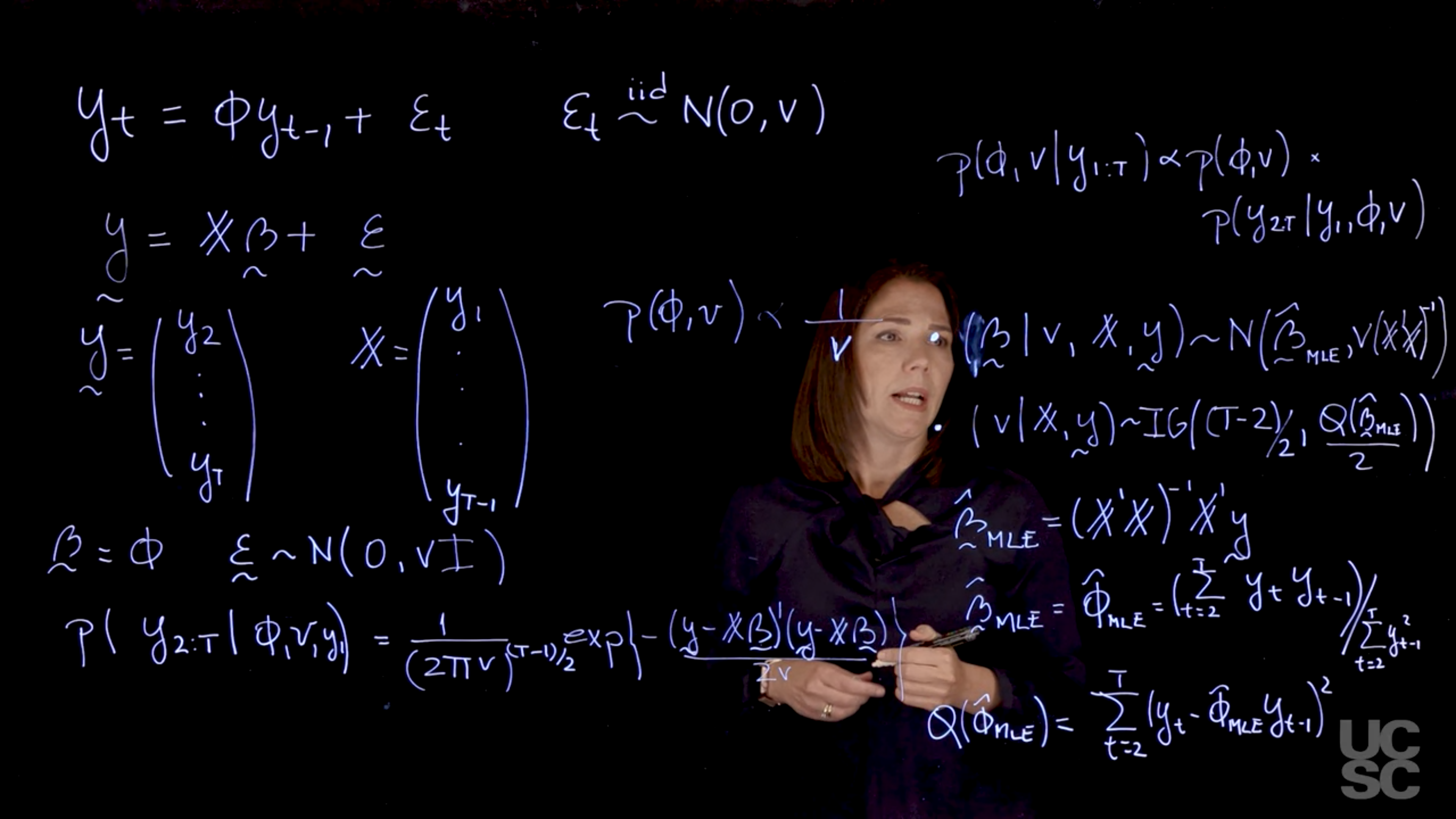{#fig-c2l1-s1-inference .column-margin group="slides" width="53mm"}
$$
y_t= \phi y_{t-1} + \varepsilon_t, \quad \varepsilon_t \overset{iid}{\sim} \mathcal{N}(0, v), \quad \phi \in (-1,1)
$$ {#eq-ar1-model}
$$
\utilde{y} = \mathbb{X}\utilde{\beta} + \utilde{\varepsilon}
$$ {#eq-ar1-model-bayes}
where $\mathbb{X}$ is the design matrix with $y_1$ as the first column and $y_2, \ldots, y_{T-1}$ as the second column, $\utilde{\beta} = \phi$ is the AR coefficient, and $\utilde{\varepsilon} \sim \mathcal{N}(0, v\mathbf{I})$ is the error term.
$$
\utilde{y} = \begin{pmatrix}
y_1 \\
y_2 \\
\vdots \\
y_{T-1}
\end{pmatrix}
$$ {#eq-utilde-y-ar1}
$$
\mathbb{X} = \begin{pmatrix}
y_1 \\
y_2 \\
\vdots \\
y_{T-1}
\end{pmatrix}
$$ {#eq-design-matrix-ar1}
$$
\utilde{\beta} = \phi
$$ {#eq-ar1-model}
$$
\utilde{\varepsilon} \sim \mathcal{N}(0, v\mathbf{I})
$$ {#eq-ar1-model-bayes}
$$
p(y_{2:T} \mid y_1, \phi, v) = \frac{1}{(2\pi v)^{\frac{T-1}{2}}} \exp\left(-\frac{(\utilde{y} - \mathbb{X}\utilde{\beta})'(\utilde{y} - \mathbb{X}\utilde{\beta})}{2v}\right)
$$ {#eq-likelihood-ar1-conditional}
$$
p(\phi, v \mid y_{1:T}) \propto p(\phi, v) p(y_{2:T} \mid y_1, \phi, v)
$$ {#eq-posterior-ar1}
$$
\begin{aligned}
p(\phi, v) \propto \frac{1}{v} &\cdot (\utilde{\beta} \mid v, \mathbb{X}, \utilde{y}) &\sim & \mathcal{N}(\hat{\utilde{\beta}}, v(\mathbb{X}'\mathbb{X})^{-1}) \\
& \cdot (v \mid \mathbb{X}, \utilde{y}) &\sim & \mathcal{IG}\left(\frac{T-2}{2}, \frac{1}{2}Q(\hat{\utilde{\beta}}_{MLE}) \right)
\end{aligned}
$$ {#eq-prior-ar1}
$$
\begin{aligned}
\hat{\utilde{\beta}_{MLE}} &= (\mathbb{X}'\mathbb{X})^{-1}\mathbb{X}'\utilde{y} \\
&= \hat{\phi}_{MLE} = \frac{\sum_{t=2}^T y_t y_{t-1}}{\sum_{t=2}^T y_{t-1}^2}
\end{aligned}
$$ {#eq-mle-ar1-phi-bayes}
$$
Q(\hat{\phi}_{MLE}) = \sum_{t=2}^T (y_t - \hat{\phi}_{MLE}\ y_{t-1})^2
$$ {#eq-q-ar1-q-mle-bayes}
::: {.callout-note collapse="true"}
## Video Transcript
{{< include transcripts/c4/01_week-1-introduction-to-time-series-and-the-ar-1-process/04_the-ar-1-maximum-likelihood-estimation-and-bayesian-inference/04_bayesian-inference-in-the-ar-1.en.txt >}}
:::
## Bayesian inference in the AR(1): Conditional likelihood example :movie_camera:
This video walks through the code snippet below and provides examples of how to sample from the posterior distribution of the AR coefficient $\psi$ and the variance $v$ using the conditional likelihood and a reference prior.
::: {.callout-note collapse="true"}
## Video Transcript
{{< include transcripts/c4/01_week-1-introduction-to-time-series-and-the-ar-1-process/04_the-ar-1-maximum-likelihood-estimation-and-bayesian-inference/05_bayesian-inference-in-the-ar-1-conditional-likelihood-example.en.txt >}}
:::
## AR(1) Bayesian inference, conditional likelihood example :spiral_notepad: $\mathcal{R}$
```{r}
#| label: "AR(1) inference, conditional likelihood example"
#|
####################################################
#####             MLE for AR(1)               ######
####################################################
set.seed(2021)
phi=0.9 # ar coefficient
sd=1 # innovation standard deviation
T=200 # number of time points
yt=arima.sim(n = T, model = list(ar = phi), sd = sd) # sample stationary AR(1) process

y=as.matrix(yt[2:T]) # response
X=as.matrix(yt[1:(T-1)]) # design matrix
phi_MLE=as.numeric((t(X)%*%y)/sum(X^2)) # MLE for phi
s2=sum((y - phi_MLE*X)^2)/(length(y) - 1) # Unbiased estimate for v
v_MLE=s2*(length(y)-1)/(length(y)) # MLE for v

print(c(phi_MLE,s2))
#######################################################
######     Posterior inference, AR(1)               ###
######     Conditional Likelihood + Reference Prior ###
######     Direct sampling                          ###
#######################################################

n_sample=3000   # posterior sample size

## step 1: sample posterior distribution of v from inverse gamma distribution
v_sample=1/rgamma(n_sample, (T-2)/2, sum((yt[2:T] - phi_MLE*yt[1:(T-1)])^2)/2)

## step 2: sample posterior distribution of phi from normal distribution
phi_sample=rep(0,n_sample)
for (i in 1:n_sample){
phi_sample[i]=rnorm(1, mean = phi_MLE, sd=sqrt(v_sample[i]/sum(yt[1:(T-1)]^2)))}

## plot histogram of posterior samples of phi and v
par(mfrow = c(1, 2),mar = c(3, 4, 2, 1), cex.lab = 1.3)
hist(phi_sample, xlab = bquote(phi),
     main = bquote("Posterior for "~phi),xlim=c(0.75,1.05), col='lightblue')
abline(v = phi, col = 'red')
hist(v_sample, xlab = bquote(v), col='lightblue', main = bquote("Posterior for "~v))
abline(v = sd, col = 'red')
```
::: {.callout-note collapse="false"}
## Overthinking Bayesian inference in the AR(1)
:thinking: Just pondering Why the red line (MLE estimates I presume) off center i.e. not the same as the posterior mean for $\phi$ and $v$. in this chart.
We will see a far greater discrepancy between the two in the coding assignment, where the posterior mean is very different from the MLE.
One idea is that this is due to the posterior mean being influenced by the prior distribution, while the MLE is solely based on the data. In this case, the prior is a **reference prior**, which does not have a strong influence on the posterior distribution, yet has a marked effect on the posterior mean.
:::
### Bayesian Inference in the AR(1), : full likelihood example :spiral_notepad:
We consider a prior distribution that assumes that $\phi$ and $v$ are independent:
$$
\mathbb{P}r(v) \propto \frac{1}{v},
$$
$$
\mathbb{P}r(\phi) = \frac{1}{2}, \quad \text{for } \phi \in (-1, 1),
$$
i.e., we assume a Uniform prior for $\phi \in (-1, 1)$. Combining this prior with the full likelihood in the AR(1) case, we obtain the following posterior density:
$$
\mathbb{P}r(\phi, v \mid y_{1:T}) \propto \frac{(1 - \phi^2)^{1/2} }{v^{T/2 + 1}} \exp\left(-\frac{Q^*(\phi)}{2v}\right), \quad -1 < \phi < 1,
$$
with
$$
Q^*(\phi) = y_1^2(1 - \phi^2) + \sum_{t=2}^{T} (y_t - \phi y_{t-1})^2.
$$
It is not possible to get a closed-form expression for this posterior or to perform direct simulation. Therefore, we use simulation-based Markov Chain Monte Carlo (MCMC) methods to obtain samples from the posterior distribution.
### Transformation of $\phi$
We first consider the following transformation on $\phi$:
$$
\eta = \log\left(\frac{1 - \phi}{\phi + 1}\right),
$$
so that $\eta \in (-\infty, \infty)$. The inverse transformation on $\eta$ is:
$$
\phi = \frac{1 - \exp(\eta)}{1 + \exp(\eta)}.
$$
Writing down the posterior density for $\eta$ and $v$, we obtain
$$
\mathbb{P}r(\eta, v \mid y_{1:T}) \propto\frac{ (1 - \phi^2)^{1/2} }{v^{T/2 + 1}} \exp\left(-\frac{Q^*(\phi)}{2v}\right) \cdot \frac{2 \exp(\eta)}{(1 + \exp(\eta))^2},
$$
with $\phi$ written as a function of $\eta$. We proceed to obtain samples from this posterior distribution using the MCMC algorithm outlined below. Once we have obtained $M$ samples from $\eta$ and $v$ after convergence, we can use the inverse transformation above to obtain posterior samples for $\phi$.
### MCMC Algorithm: Bayesian Inference for AR(1), Full Likelihood
**Algorithm**:
1. Initialize $\eta^{(0)}$ and $\beta^{(0)}$.
2. For $m$ in $1:M$ do:
- Sample $v^{(m)} \sim \text{IG}\left(\frac{T}{2}, \frac{Q^*(\phi^{(m-1)})}{2}\right)$.
- Sample $\eta^{(m)}$ using Metropolis-Hastings:
1. Sample $\eta^* \sim N(\eta^{(m-1)}, c)$, where $c$ is a tuning parameter.
2. Compute the importance ratio:
$$
r = \frac{p(\eta^*, v^{(m)} \mid y_{1:T})}{p(\eta^{(m-1)}, v^{(m)} \mid y_{1:T})}.
$$
3. Set:
$$
\eta^{(m)} =
\begin{cases}
\eta^* & \text{with probability } \min(r, 1), \\
\eta^{(m-1)} & \text{otherwise}.
\end{cases}
$$


 inference, conditional likelihood example-1.png)