set.seed(32) # Initializes the random number generator so we can replicate these results. To get different random numbers, change the seed.
m = 100
a = 2.0
b = 1.0 / 3.0 32.1 Monte Carlo Integration 🎥
Before we learn how to simulate from complicated posterior distributions, let’s review some of the basics of Monte Carlo estimation.
Monte Carlo estimation refers to simulating hypothetical draws from a probability distribution in order to calculate important quantities. By “important quantities,” we mean things like the mean, the variance, or the probability of some event or distributional property.
All of these calculations involve integration, which except for the simplest distributions, may range from very difficult to impossible :-) .
Suppose we have a random variable \theta that follows a \Gamma distribution
\theta \sim \mathrm{Gamma}(a,b) \qquad \tag{32.1}
Let’s say a=2 and b=\frac{1}{3} , where a is the shape parameter and b is the rate parameter.
a=2 \qquad b=1/3 \qquad \tag{32.2}
To calculate the mean of this distribution, we would need to compute the following integral. It is possible to compute this integral, and the answer is \frac{a}{b} (6 in this case).
\mathbb{E}[\theta] = \int_0^\infty \theta f(\theta) d\theta = \int_0^\infty \theta \frac{b^a}{\Gamma(a)}\theta^{a-1}e^{-b\theta} d\theta = \frac{a}{b} \qquad \tag{32.3}
However, we could verify this answer through Monte Carlo estimation.
To do so, we would simulate a large number of draws (call them \theta^∗_i \quad (i=1,\ldots ,m) ) from this gamma distribution and calculate their sample mean.
Why can we do this?
Recall from the previous course that if we have a random sample from a distribution, the average of those samples converges in probability to the true mean of that distribution by the Law of Large Numbers.
Furthermore, by the Central Limit Theorem (CLT), this sample mean \bar{\theta}^* = \frac{1}{m}\sum_{i=1}^m \theta_i^* approximately follows a normal distribution with mean \mathbb{E}[\theta] and variance \mathbb{V}ar[\theta]/m .
The theoretical variance of \theta is the following integral:
\text{Var}[\theta] = \int_0^\infty (\theta-\mathbb{E}(\theta))^2 f(\theta) d\theta \qquad \tag{32.4}
Just like we did with the mean, we could approximate this variance with the sample variance
\text{Var}[\theta^*] = \frac{1}{m}\sum_{i=1}^m (\theta_i^* - \bar{\theta}^*)^2 \qquad \tag{32.5}
32.1.1 Calculating probabilities
This method can be used to calculate many different integrals. Say h(\theta) is any function and we want to calculate
\int h(\theta) \mathbb{P}r(\theta) d\theta = \mathbb{E}(h(\theta)) \approx \frac{1}{m}\sum_{i=1}^m h(\theta_i^*) \qquad \tag{32.6}
where \mathbb{P}r(\theta) is the probability density function of \theta and h(\theta) is any function of \theta.
This integral is precisely what is meant by \mathbb{E}[h(\theta)] , so we can conveniently approximate it by taking the sample mean of h(\theta_i^*). That is, we apply the function h to each simulated sample from the distribution, and take the average of all the results.
One extremely useful example of an h function is is the indicator I_A(\theta) where A is some logical condition about the value of \theta. To demonstrate, suppose h(\theta)=I_{[\theta<5]}(\theta), which will give a 1 if \theta <5 and return a 0 otherwise.
What is \mathbb{E}(h(\theta))?
This is the integral:
\begin{aligned} \mathbb{E}[h(\theta)] &= \int_0^\infty \mathbb{I}_{[\theta<5]}(\theta) \mathbb{P}r(\theta) d\theta \\ &= \int_0^5 1 \cdot \mathbb{P}r(\theta) d\theta + \int_5^\infty 0 \cdot \mathbb{P}r(\theta) d\theta \\ &= \mathbb{P}r(\theta < 5) \qquad \end{aligned} \tag{32.7}
So what does this mean?
It means we can approximate the probability that \theta < 5 by drawing many samples \theta^∗_i , and approximating this integral with \frac{1}{m} \sum_{i=1}^m I_{\theta^* < 5} (\theta_i^*). This expression is simply counting how many of those samples come out to be less than 5 , and dividing by the total number of simulated samples.
That’s convenient!
Likewise, we can approximate quantiles of a distribution. If we are looking for the value z such that \mathbb{P}r(\theta < z) = 0.9 , we simply arrange the samples \theta^∗_i in ascending order and find the smallest drawn value that is greater than 90% of the others.
32.2 Monte Carlo Error and Marginalization
How good is an approximation by Monte Carlo sampling?
Again we can turn to the Central Limit Theorem, which tells us that the variance of our estimate is controlled in part by m. For a better estimate, we want larger m.
For example, if we seek \mathbb{E}[\theta] , then the sample mean \bar\theta^∗ approximately follows a normal distribution with mean \mathbb{E}[\theta] and variance Var[\theta]/m .
The variance tells us how far our estimate might be from the true value.
One way to approximate \mathbb{V}ar[\theta] is to replace it with the sample variance.
The standard deviation of our Monte Carlo estimate is the square root of that, or the sample standard deviation divided by \sqrt{m} .
If m is large, it is reasonable to assume that the true value will likely be within about two standard deviations of your Monte Carlo estimate.
32.3 Marginalization
We can also obtain Monte Carlo samples from hierarchical models.
As a simple example, let’s consider a binomial random variable where y \mid \phi \sim \mathrm{Bin}(10,\phi) and further suppose \phi is random (as if it had a prior) and is distributed beta \phi \sim \mathrm{Beta}(2,2) .
Given any hierarchical model, we can always write the joint distribution of y and \phi as \mathbb{P}r(y,\phi) = \mathbb{P}r(y \mid \phi)\mathbb{P}r(\phi) using the chain rule of probability.
To simulate from this joint distribution, repeat these steps for a large number m :
- Simulate \phi^∗_i from its Beta(2,2) distribution.
- Given the drawn \phi^∗_i , simulate y^∗_i from Bin(10,\phi^*_i) .
This will produce m independent pairs of (y^∗,\phi^∗)_i drawn from their joint distribution.
One major advantage of Monte Carlo simulation is that marginalizing is easy. Calculating the marginal distribution of y , \mathbb{P}r(y)=\int^1_0 \mathbb{P}r(y,\phi)d\phi, might be challenging. But if we have draws from the joint distribution, we can just discard the \phi^∗_i draws and use the y^∗_i as samples from their marginal distribution.
This is also called the prior predictive distribution introduced in the previous course.
In the next segment, we will demonstrate some of these principles.
Remember, we do not yet know how to sample from the complicated posterior distributions introduced in the previous lesson.
But once we learn that, we will be able to use the principles from this lesson to make approximate inferences from those posterior distributions.
32.4 Computing Examples
Monte Carlo simulation from the most common distributions is very straightforward in R.
Let’s start with the example from the previous segment, where \theta \sim Gamma(a,b) with a=2, b=1/3 . This could represent the posterior distribution of \theta if our data came from a Poisson distribution with mean \theta and we had used a conjugate gamma prior. Let’s start with m=100 .
To simulate m independent samples, use the rgamma function.
theta <- rgamma(n=m, shape = a, rate=b) We can plot a histogram of the generated data, and compare that to the true density.
hist(theta, freq=FALSE)
curve(dgamma(x=x, shape=a, rate=b), col="blue", add=TRUE)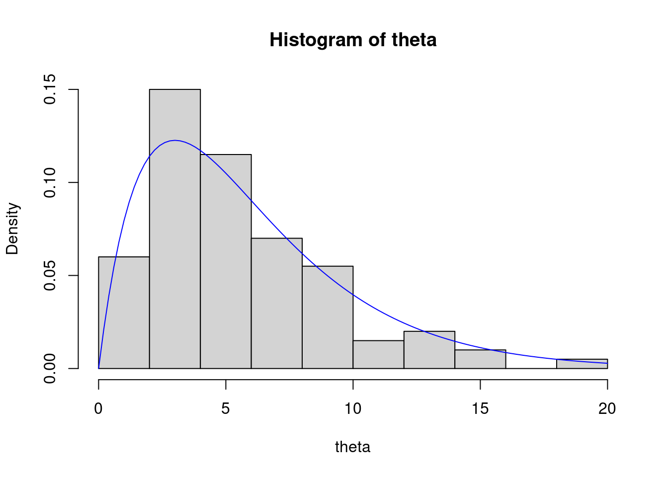
To find our Monte Carlo approximation to \mathbb{E}(\theta) , let’s take the average of our sample (and compare it with the truth).
sum(theta) / m # sample mean [1] 5.514068mean(theta) # sample mean [1] 5.514068a / b # true expected value[1] 6Not bad, but we can do better if we increase m to say, 10,000.
m = 1e4
theta = rgamma(n=m, shape=a, rate=b)
mean(theta)
[1] 6.023273How about the variance of \theta ?
var(theta) # sample variance[1] 18.04318a / b^2 # true variance of Gamma(a,b) [1] 18We can also approximate the probability that \theta < 5 .
ind = theta < 5.0 # set of indicators, TRUE if theta_i < 5
mean(ind)         # automatically converts FALSE/TRUE to 0/1
[1] 0.497pgamma(q=5.0, shape=a, rate=b) # true value of Pr( theta < 5 )[1] 0.4963317What is the 0.9 quantile (90th percentile) of \theta ? We can use the quantile function which will order the samples for us and find the appropriate sample quantile.
quantile(x=theta, probs=0.9) 90%
11.74338 qgamma(p=0.9, shape=a, rate=b) # true value of 0.9 quantile[1] 11.6691632.5 Monte Carlo error
We can use the Central limit theorem to approximate how accurate our Monte Carlo estimates are. For example, if we seek E(\theta) , then the sample mean \bar\theta^∗ approximately follows a normal distribution with mean \mathbb{E}(\theta) and variance Var(\theta)/m . We will use the sample standard deviation divided by the square root of m to approximate the Monte Carlo standard deviation.
se = sd(theta) / sqrt(m)
2.0 * se # we are reasonably confident that the Monte Carlo estimate is no more than this far from the truth
[1] 0.08495454These numbers give us a reasonable range for the quantity we are estimating with Monte Carlo. The same applies for other Monte Carlo estimates, like the probability that \theta < 5.
ind = theta < 5.0
se = sd(ind) / sqrt(m)
2.0 * se # we are reasonably confident that the Monte Carlo estimate is no more than this far from the truth
[1] 0.0100003232.6 Marginalization
Let’s also do the second example of simulating a hierarchical model. In our example from the previous segment, we had a binomial random variable where y \mid \phi \overset{\text{iid}}{\sim}\text{Binomial}(10,\phi), and \phi \sim Beta(2,2). To simulate from this joint distribution, repeat these steps for a large number m :
- Simulate \phi_i from its Beta(2,2) distribution.
- Given the drawn \phi_i , simulate y_i from Bin(10,\phi_i) .
m = 10e4

y = numeric(m) # create the vectors we will fill in with simulations
phi = numeric(m)

for (i in 1:m) {
  phi[i] = rbeta(n=1, shape1=2.0, shape2=2.0)
  y[i] = rbinom(n=1, size=10, prob=phi[i])
}
# which is equivalent to the following 'vectorized' code
phi = rbeta(n=m, shape1=2.0, shape2=2.0)
y = rbinom(n=m, size=10, prob=phi)
If we are interested only in the marginal distribution of y , we can just ignore the draws for \phi and treat the draws of y as a sample from its marginal distribution.
mean(y) [1] 5.00008plot(prop.table(table(y)), ylab="Pr(y)", main="Marginal distribution of y")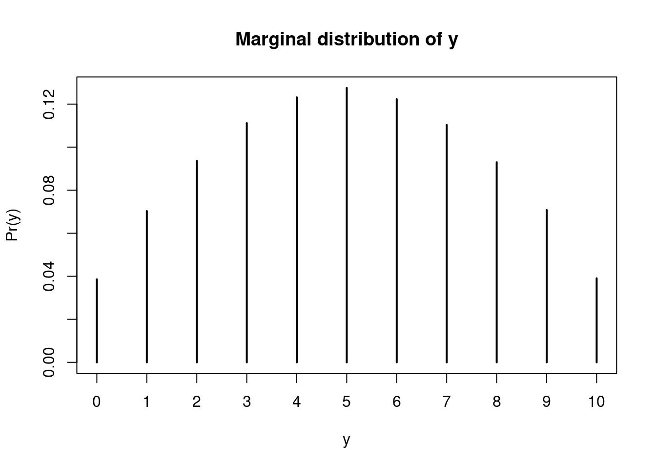
33 Markov chains
33.1 Definition
If we have a sequence of random variables X_1,X_2,\dots X_n where the indices 1,2,\dots,n represent successive points in time, we can use the chain rule of probability to calculate the probability of the entire sequence:
\mathbb{P}r(X_1, X_2, \ldots X_n) = \mathbb{P}r(X_1) \cdot \mathbb{P}r(X_2 \mid X_1) \cdot \mathbb{P}r(X_3 \mid X_2, X_1) \cdot \ldots \cdot \mathbb{P}r(X_n \mid X_{n-1}, X_{n-2}, \ldots, X_2, X_1) \qquad \tag{33.1}
Markov chains simplify this expression by using the Markov assumption. The assumption is that given the entire past history, the probability distribution for the random variable at the next time step only depends on the current variable. Mathematically, the assumption is written like this:
\mathbb{P}r(X_{t+1} \mid X_t, X_{t-1}, \ldots, X_2, X_1 ) = \mathbb{P}r(X_{t+1} \mid X_t) \qquad \tag{33.2}
for all t=2,\dots,n. Under this assumption, we can write the first expression as
\mathbb{P}r(X_1, X_2, \ldots X_n) = \mathbb{P}r(X_1) \cdot \mathbb{P}r(X_2 \mid X_1) \cdot \mathbb{P}r(X_3 \mid X_2) \cdot \mathbb{P}r(X_4 \mid X_3) \cdot \ldots \cdot \mathbb{P}r(X_n \mid X_{n-1}) \qquad \tag{33.3}
which is much simpler than the original. It consists of an initial distribution for the first variable, \mathbb{P}r(X_1), and n−1 transition probabilities. We usually make one more assumption: that the transition probabilities do not change with time. Hence, the transition from time t to time t+1 depends only on the value of Xt.
33.2 Examples of Markov chains
33.2.1 Discrete Markov chain
Suppose you have a secret number (make it an integer) between 1 and 5. We will call it your initial number at step 1. Now for each time step, your secret number will change according to the following rules:
- Flip a coin.
- If the coin turns up heads, then increase your secret number by one (5 increases to 1).
- If the coin turns up tails, then decrease your secret number by one (1 decreases to 5).
- Repeat n times, and record the evolving history of your secret number.
Before the experiment, we can think of the sequence of secret numbers as a sequence of random variables, each taking on a value in \{1,2,3,4,5\}. Assume that the coin is fair, so that with each flip, the probability of heads and tails are both 0.5.
Does this game qualify as a true Markov chain? Suppose your secret number is currently 4 and that the history of your secret numbers is (2,1,2,3). What is the probability that on the next step, your secret number will be 5? What about the other four possibilities? Because of the rules of this game, the probability of the next transition will depend only on the fact that your current number is 4. The numbers further back in your history are irrelevant, so this is a Markov chain.
This is an example of a discrete Markov chain, where the possible values of the random variables come from a discrete set. Those possible values (secret numbers in this example) are called states of the chain. The states are usually numbers, as in this example, but they can represent anything. In one common example, the states describe the weather on a particular day, which could be labeled as 1-fair, 2-poor.
33.2.2 Random walk (continuous)
Now let’s look at a continuous example of a Markov chain. Say X_t=0 and we have the following transition model:
\mathbb{P}r(X_{t+1}\mid X_t=x_t)=N(x_t,1) \qquad \tag{33.4}
That is, the probability distribution for the next state is Normal with variance 1 and mean equal to the current state. This is often referred to as a “random walk.” Clearly, it is a Markov chain because the transition to the next state Xt+1 only depends on the current state Xt.
This example is straightforward to code in R:
set.seed(34)

n = 100
x = numeric(n)

for (i in 2:n) {
  x[i] = rnorm(1, mean=x[i-1], sd=1.0)
}

plot.ts(x)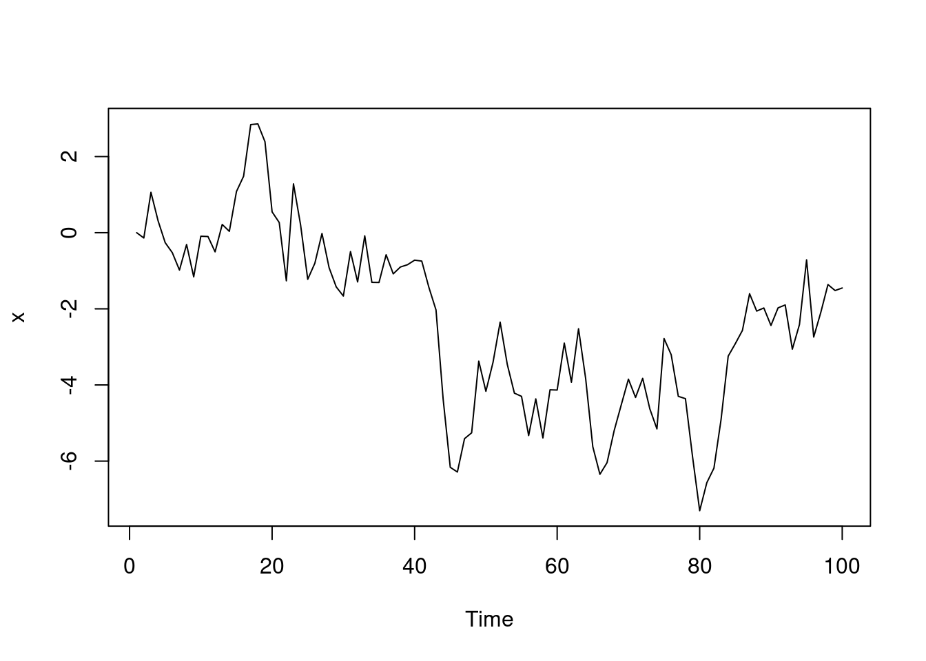
33.3 Transition matrix
Let’s return to our example of the discrete Markov chain. If we assume that transition probabilities do not change with time, then there are a total of 25 (52) potential transition probabilities. Potential transition probabilities would be from State 1 to State 2, State 1 to State 3, and so forth. These transition probabilities can be arranged into a matrix Q:
Q = \begin{pmatrix} 0 & .5 & 0 & 0 & .5 \\ .5 & 0 & .5 & 0 & 0 \\ 0 & .5 & 0 & .5 & 0 \\ 0 & 0 & .5 & 0 & .5 \\ .5 & 0 & 0 & .5 & 0 \\ \end{pmatrix} \qquad \tag{33.5}
where the transitions from State 1 are in the first row, the transitions from State 2 are in the second row, etc. For example, the probability \mathbb{P}r(X_{t+1}=5\mid X_t=4) can be found in the fourth row, fifth column.
The transition matrix is especially useful if we want to find the probabilities associated with multiple steps of the chain. For example, we might want to know \mathbb{P}r(X_{t+2}=3 \mid X_t=1), the probability of your secret number being 3 two steps from now, given that your number is currently 1. We can calculate this as \sum_{k=15} \mathbb{P}r(X_t+2=3 \mid X_t+1=k) \cdot \mathbb{P}r(X_{t+1}=k \mid X_t=1), which conveniently is found in the first row and third column of Q_2.
We can perform this matrix multiplication easily in R:
Q = matrix(c(0.0, 0.5, 0.0, 0.0, 0.5,
             0.5, 0.0, 0.5, 0.0, 0.0,
             0.0, 0.5, 0.0, 0.5, 0.0,
             0.0, 0.0, 0.5, 0.0, 0.5,
             0.5, 0.0, 0.0, 0.5, 0.0),
           nrow=5, byrow=TRUE)

Q %*% Q # Matrix multiplication in R. This is Q^2.
[,1] [,2] [,3] [,4] [,5]
[1,] 0.50 0.00 0.25 0.25 0.00
[2,] 0.00 0.50 0.00 0.25 0.25
[3,] 0.25 0.00 0.50 0.00 0.25
[4,] 0.25 0.25 0.00 0.50 0.00
[5,] 0.00 0.25 0.25 0.00 0.50(Q %*% Q)[1,3][1] 0.25Therefore, if your secret number is currently 1, the probability that the number will be 3 two steps from now is .25.
33.4 Stationary distribution
Suppose we want to know the probability distribution of the your secret number in the distant future, say \mathbb{P}r(X_{t+h} \mid X_t) where h is a large number. Let’s calculate this for a few different values of h.
Q5 = Q %*% Q %*% Q %*% Q %*% Q # h=5 steps in the future
round(Q5, 3)
[,1] [,2] [,3] [,4] [,5]
[1,] 0.062 0.312 0.156 0.156 0.312
[2,] 0.312 0.062 0.312 0.156 0.156
[3,] 0.156 0.312 0.062 0.312 0.156
[4,] 0.156 0.156 0.312 0.062 0.312
[5,] 0.312 0.156 0.156 0.312 0.062Q10 = Q %*% Q %*% Q %*% Q %*% Q %*% Q %*% Q %*% Q %*% Q %*% Q # h=10 steps in the future
round(Q10, 3) [,1] [,2] [,3] [,4] [,5]
[1,] 0.248 0.161 0.215 0.215 0.161
[2,] 0.161 0.248 0.161 0.215 0.215
[3,] 0.215 0.161 0.248 0.161 0.215
[4,] 0.215 0.215 0.161 0.248 0.161
[5,] 0.161 0.215 0.215 0.161 0.248Q30 = Q
for (i in 2:30) {
Q30 = Q30 %*% Q
}
round(Q30, 3) # h=30 steps in the future [,1] [,2] [,3] [,4] [,5]
[1,] 0.201 0.199 0.200 0.200 0.199
[2,] 0.199 0.201 0.199 0.200 0.200
[3,] 0.200 0.199 0.201 0.199 0.200
[4,] 0.200 0.200 0.199 0.201 0.199
[5,] 0.199 0.200 0.200 0.199 0.201Notice that as the future horizon gets more distant, the transition distributions appear to converge. The state you are currently in becomes less important in determining the more distant future. If we let h get really large, and take it to the limit, all the rows of the long-range transition matrix will become equal to (.2,.2,.2,.2,.2). That is, if you run the Markov chain for a very long time, the probability that you will end up in any particular state is 1/5=.2 for each of the five states. These long-range probabilities are equal to what is called the stationary distribution of the Markov chain.
The stationary distribution of a chain is the initial state distribution for which performing a transition will not change the probability of ending up in any given state. That is,
c(0.2, 0.2, 0.2, 0.2, 0.2) %*% Q [,1] [,2] [,3] [,4] [,5]
[1,] 0.2 0.2 0.2 0.2 0.2One consequence of this property is that once a chain reaches its stationary distribution, the stationary distribution will remain the distribution of the states thereafter.
We can also demonstrate the stationary distribution by simulating a long chain from this example.
n = 5000
x = numeric(n)
x[1] = 1 # fix the state as 1 for time 1
for (i in 2:n) {
  x[i] = sample.int(5, size=1, prob=Q[x[i-1],]) # draw the next state from the intergers 1 to 5 with probabilities from the transition matrix Q, based on the previous value of X.
}
Now that we have simulated the chain, let’s look at the distribution of visits to the five states.
table(x) / nx
1 2 3 4 5
0.1996 0.2020 0.1980 0.1994 0.2010 The overall distribution of the visits to the states is approximately equal to the stationary distribution.
As we have just seen, if you simulate a Markov chain for many iterations, the samples can be used as a Monte Carlo sample from the stationary distribution. This is exactly how we are going to use Markov chains for Bayesian inference. In order to simulate from a complicated posterior distribution, we will set up and run a Markov chain whose stationary distribution is the posterior distribution.
It is important to note that the stationary distribution doesn’t always exist for any given Markov chain. The Markov chain must have certain properties, which we won’t discuss here. However, the Markov chain algorithms we’ll use in future lessons for Monte Carlo estimation are guaranteed to produce stationary distributions.
33.4.1 Continuous example
The continuous random walk example we gave earlier does not have a stationary distribution. However, we can modify it so that it does have a stationary distribution.
Let the transition distribution be \mathbb{P}r(X_{t + 1}\mid X_t = x_t)=N(\phi x_t,1) where -1 < \phi < 1. That is, the probability distribution for the next state is Normal with variance 1 and mean equal to \phi times the current state. As long as \phi is between −1 and 1, then the stationary distribution will exist for this model.
Let’s simulate this chain for \phi=−0.6.
set.seed(38)

n = 1500
x = numeric(n)
phi = -0.6

for (i in 2:n) {
  x[i] = rnorm(1, mean=phi*x[i-1], sd=1.0)
}

plot.ts(x)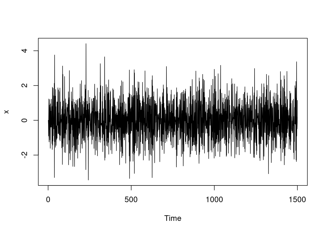
The theoretical stationary distribution for this chain is normal with mean 0 and variance 1/(1−\phi^2), which in our example approximately equals 1.562. Let’s look at a histogram of our chain and compare that with the theoretical stationary distribution.
\text{Var}_{\text{stationary}} = \frac{1}{1-\phi^2} \qquad \tag{33.6}
hist(x, freq=FALSE)
curve(dnorm(x, mean=0.0, sd=sqrt(1.0/(1.0-phi^2))), col="red", add=TRUE)
legend("topright", legend="theoretical stationary\ndistribution", col="red", lty=1, bty="n")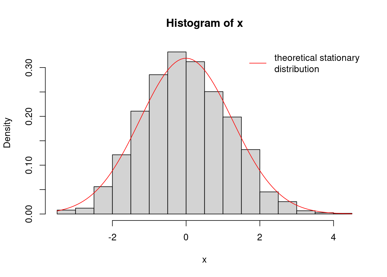
It appears that the chain has reached the stationary distribution. Therefore, we could treat this simulation from the chain like a Monte Carlo sample from the stationary distribution, a normal with mean 0 and variance 1.562.
Because most posterior distributions we will look at are continuous, our Monte Carlo simulations with Markov chains will be similar to this example.