21 M4L9 - Exponential Data

21.1 Exponential Data

Figure 21.1: Exponential likelihood with a Gamma prior

Suppose you’re waiting for a bus that you think comes on average once every 10 minutes, but you’re not sure exactly how often it comes.

Time between buses

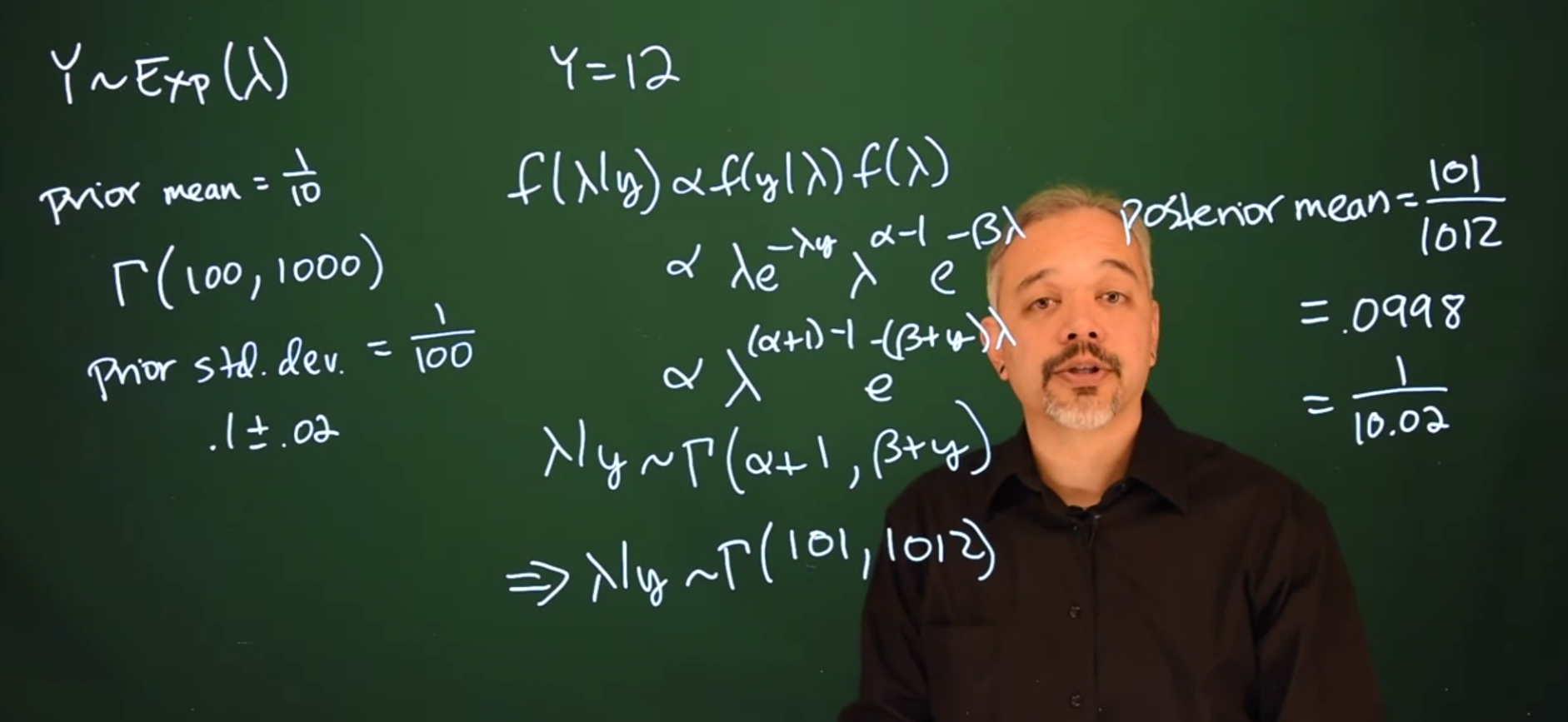
Y \sim \mathrm{Exp}(\lambda) \tag{21.1}

Your waiting time has a prior expectation of \frac{1}{\lambda}

The Gamma distribution is conjugate for an Exponential likelihood. We need to specify a prior, or a particular Gamma in this case. If we think that the buses come on average every ten minutes, that’s a rate of one over ten.

prior_{\mu} = \frac{1}{10}

Thus, we’ll want to specify a gamma distribution so that the first parameter divided by the second parameter is {1 \over 10}

We can now think about our variability. Perhaps you specify

\mathrm{Gamma}(100, 1000)

This will indeed have a prior mean of {1 \over 10} and it’ll have a standard deviation of {1 \over 100}. If you want to have a rough estimate of our mean plus or minus two standard deviations then we have the following

0.1 \pm 0.02

Suppose that we wait for 12 minutes and a bus arrives. Now you want to update your posterior for \lambda about how often this bus will arrive.

f(\lambda \mid y) \propto f(y\mid \lambda)f(\lambda)

f(\lambda \mid y) \propto \lambda e^{-\lambda y}\lambda^{\alpha - 1}e^{-\beta \lambda}

f(\lambda \mid y) \propto \lambda^{(\alpha + 1) - 1}e^{-(\beta + y)\lambda}

\lambda \mid y \sim \mathrm{Gamma}(\alpha + 1, \beta + y)

Plugging in our particular prior gives us a posterior for \lambda which is

\lambda \mid y \sim \mathrm{Gamma}(101, 1012)

Thus our posterior mean is going to be \frac{101}{1012} = 0.0998.

This one observation does not contain a lot of data under this likelihood. When the bus comes and it takes 12 minutes instead of 10, it barely shifts our posterior mean up.

One data point does not have a big impact here.

Exercise 21.1 We can generalize the result from the lesson to more than one data point.

Suppose

Y_1, \ldots, Y_n \stackrel{iid}\sim Exp(\lambda)=\lambda e^{-\lambda x}\mathbb{I}_{x\ge0}

with mean

\mathbb{E}[Y]=\frac{1}{\lambda}

and assume a

f(\lambda)= \mathrm{Gamma}(\alpha, \beta) \qquad (\text{prior for }\lambda)

The likelihood is then:

f(y \mid \lambda) = \prod \lambda e^{-\lambda x}\mathbb{I}_{x\ge0} = \lambda ^ n e^{− \lambda \sum y_i}\cdot1

and we can follow the same steps from the lesson to obtain the posterior distribution (try to derive it yourself):

\lambda \mid y ∼ \mathrm{Gamma}(\alpha + n, \beta + \sum y_i)

What is the prior effective sample size (ess) in this model?

Solution. The data sample size n is added to \alpha to update the first parameter. Thus \alpha can be interpreted as the sample size equivalent in the prior.

It might be helpful to think about a related problems…

1. We are waiting at a bus stop with 1 bus line, the information at the bus stop say that the bus comes on average every 10 minutes at this time. How long do we expect to wait for the bus?
2. what if we have waited for k minutes and the bus has not arrived yet? How long do we expect to wait for the bus?
3. While we are waiting more people arrive at the bus stop. You notice the bus stop features a digital counter and a display with long term mean E and V variance of the number of people at the bus stop. Can we use this information to get a better estimate of our bus arrival time?
4. If we wait at a bus stop with K different bus lines each with the same lambda, and we see a L people waiting. Can we get a better estimate of our bus arrival time?
5. What if more people come. And we know the mean and variance of the people waiting at the bus stop?
6. What if a different bus line arrives and the number of people waiting is now M?
7. What if each bus line has a different lambda, but we know the mean and variance of the people waiting at the bus stop?