---
date: 2024-11-02
title: "The AR(1) process: definitions and properties - M1L2"
subtitle: Time Series Analysis
description: "This lesson we will define the AR(1) process, Stationarity, ACF, PACF, differencing, smoothing"
categories:
- coursera
- notes
- bayesian statistics
- autoregressive models
- time series
keywords:
- AR(1) process
- Yule-Walker equations
- Durbin-Levinson recursion
- R code
---
::: {.callout-note collapse="true"}
## Learning Objectives
- [x] Define the zero-mean autoregressive process of order one or *AR(1)* [\#](#l2g1)
- [x] use R to obtain samples from this type of process. [\#](#l2g2)
- [x] Perform maximum likelihood estimation for the full and conditional likelihood in an AR(1) [\#](#l2g3)
:::
We will next introduce the autoregressive process of order one, or *AR(1)* process, which is a fundamental model in time series analysis. We will discuss the definition of the *AR(1)* process, its properties, and how to simulate data from an *AR(1)* process.
## The AR(1) process :movie_camera:
{#fig-c4l3-s1 .column-margin group="slides" width="53mm"}
{#fig-c4l3-s2 .column-margin group="slides" width="53mm"}
### AR(1) Definition {#sec-ar1-definition}
\index{AR(1)!definition}
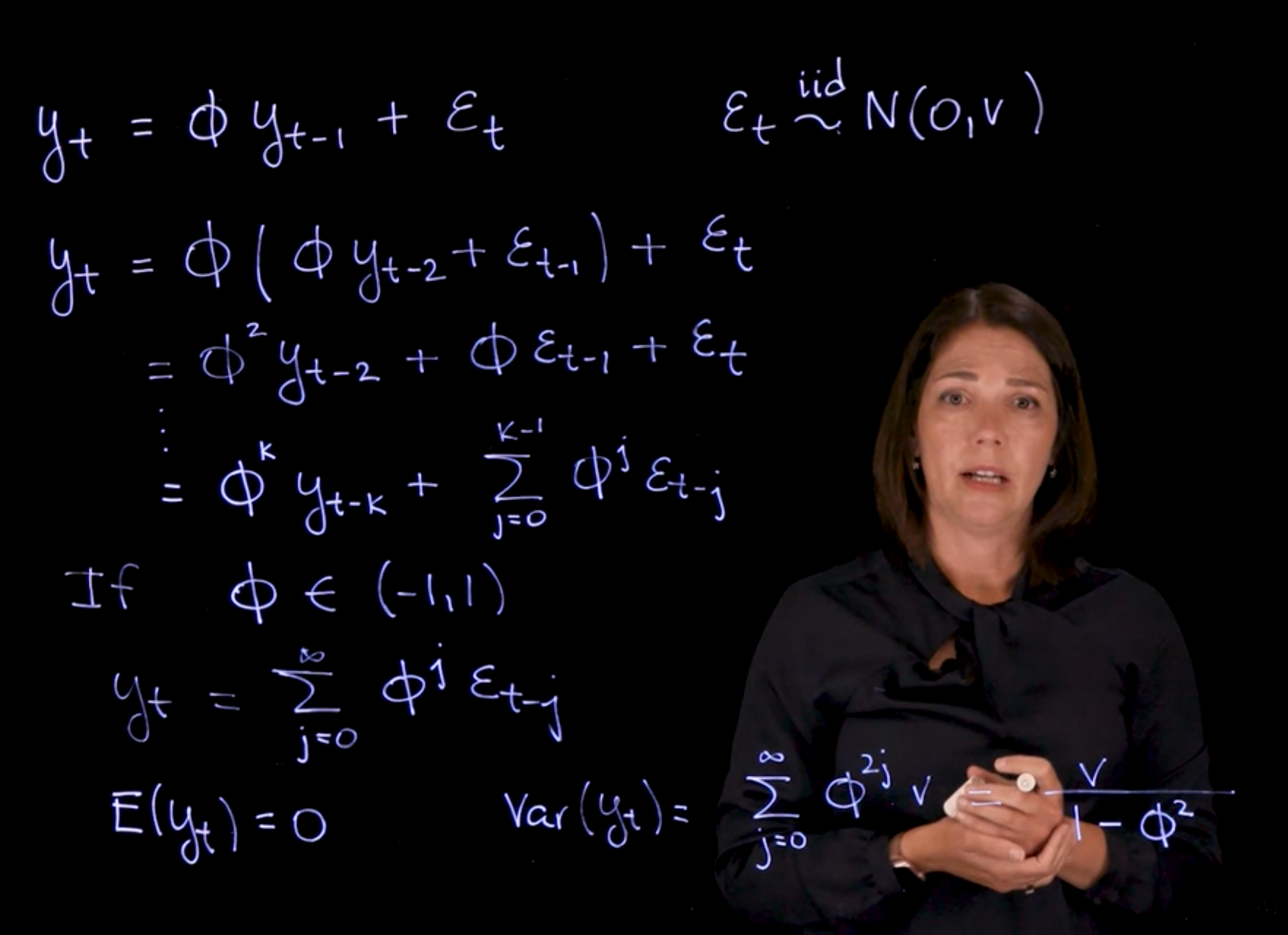
[The AR(1) process is defined as]{#l2g1 .mark}:
$$
y_t = \phi y_{t-1} + \varepsilon_t \qquad \varepsilon_t \overset{iid}{\sim} \mathcal{N}(0, v)
$$ {#eq-ar1-definition}
- where:
- $\phi$ is the *AR(1)* coefficient
- $\varepsilon_t$ are the innovations (or shocks) at time $t$, assumed to be independent and identically distributed (i.i.d.) with mean 0 and variance $v$.
### AR(1) Recursive Expansion
Recursive substitution yields:
$$
\begin{aligned}
y_t &= \phi(\phi y_{t-1} )+ \varepsilon_t \\
&= \phi^2 y_{t-2} + \phi \varepsilon_{t-1} + \varepsilon_t \\
&= \phi^k y_{t-k} + \sum_{j=0}^{k-1} \phi^j \varepsilon_{t-j}
\end{aligned}
$$ {#eq-ar1-recursive}
For $\|\phi\| < 1$, as $k \to \infty$, this becomes:
$$
y_t = \sum_{j=0}^{\infty} \phi^j \varepsilon_{t-j}
$$ {#eq-ar1-infinite-expansion}
Interpreted as an infinite-order **Moving Average** $\operatorname{MA}(\infty)$ process.
### AR(1) Mean
\index{AR(1)!mean}
Since $\mathbb{E}[\varepsilon_t] = 0$,
$$
\mathbb{E}[y_t] = 0 \text{ mean of the AR(1) process}
$$ {#eq-ar1-mean}
### AR(1) Variance
\index{AR(1)!variance}
Using independence and identical distribution:
$$
\mathbb{V}ar[y_t] = \sum_{j=0}^{\infty} \phi^{2j} v = \frac{v}{1 - \phi^2}
$$ {#eq-ar1-variance}
Requires $\|\phi\| < 1$ for convergence (i.e., stationarity).
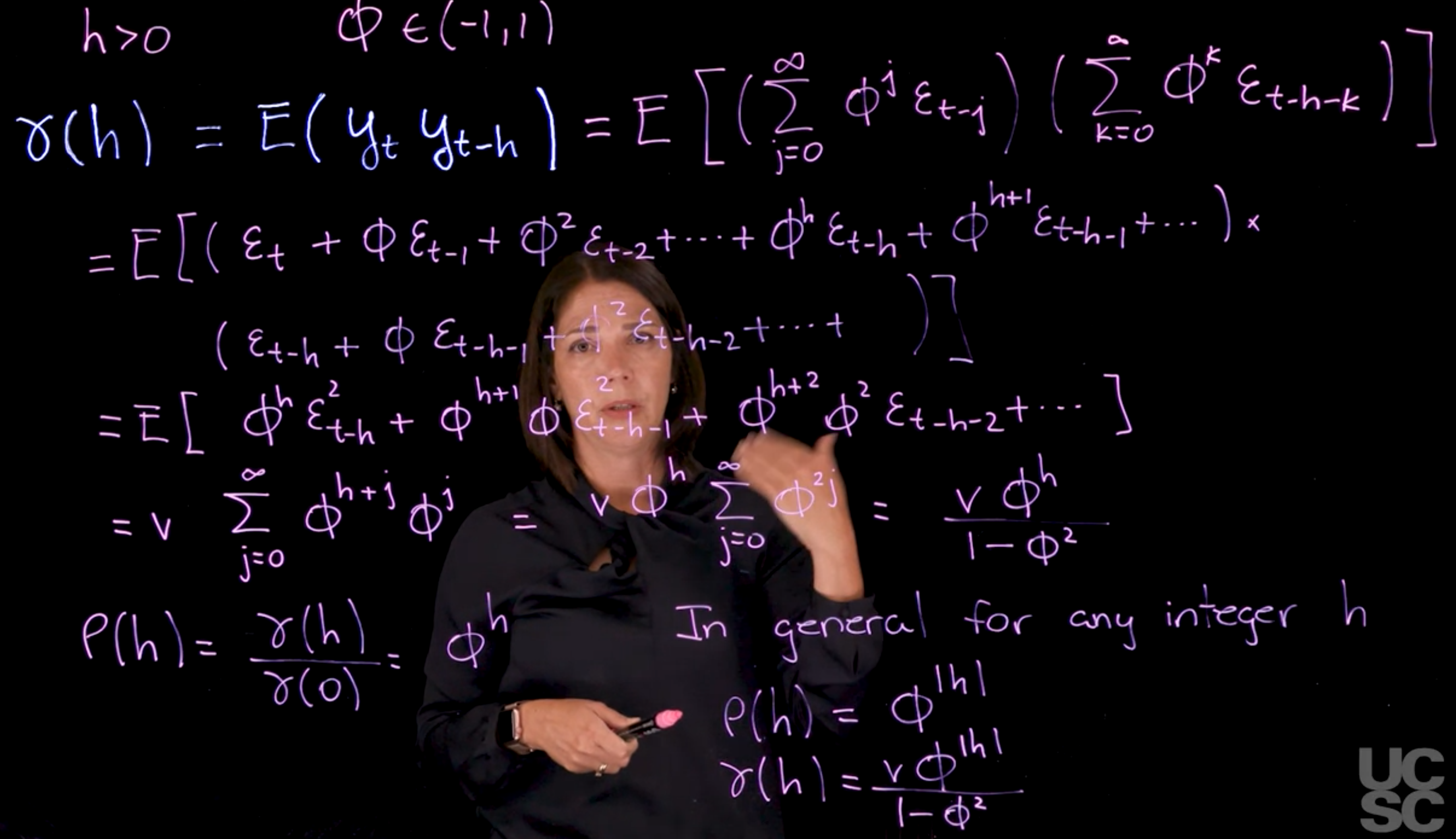
### AR(1) Autocovariance Function $\gamma(h)$
\index{AR(1)!autocovariance}
For lag $h$, the autocovariance:
$$
\begin{aligned}
\gamma(h) &= \mathbb{E}[y_t y_{t-h}] \\
&= \mathbb{E} \left[ \left( \sum_{j=0}^{\infty} \phi^j \varepsilon_{t-j}\right )\left (\sum_{k=0}^{\infty} \phi^k \varepsilon_{t-h-k}\right) \right] \\
&= \mathbb{E}[(\varepsilon_{t} + \phi \varepsilon_{t-1} + \phi^2 \varepsilon_{t-2} + \ldots ) \times (\varepsilon_{t-h} + \phi \varepsilon_{t-h-1} + \phi^2 \varepsilon_{t-h-2} + \ldots ) ] \\
&= \mathbb{E}[\phi ^h \varepsilon_{t-h} \varepsilon_{t} + \phi^{h+1} \varepsilon_{t-h-1} \varepsilon_{t} + \ldots] \\
&= v \sum_{j=0}^{\infty} \phi^{h+j} \phi^{j} \\
&= v \phi^h \sum_{j=0}^{\infty} \phi^{2j} \\
&= \frac{v \phi^{\|h\|}}{1 - \phi^2} \qquad \text { when } |\phi| < 1
\end{aligned}
$$ {#eq-ar1-autocovariance}
We used the definition and properties of the expectation, independence of the innovations $\varepsilon_t$, and the fact that $\mathbb{E}[\varepsilon_t^2] = v$.
In the cross product, only terms where lags are the same ($j = k$) contribute, as the others are independent, leading to the above result. In the final step, we used the formula for the sum of a geometric series.
### AR(1) Autocorrelation Function $\rho(h)$
\index{AR(1)!ACF}
\index{AR(1)!PACF}
Defined by:
$$
\rho(h) = \frac{\gamma(h)}{\gamma(0)} = \phi^{\|h\|}
$$ {#eq-ar1-autocorrelation}
### AR(1) other properties:
1. for any lag $h$:
- $\rho(h) = \phi^{\|h\|}$
- $\gamma(h) = \frac{v \phi^{\|h\|}}{1 - \phi^2}$
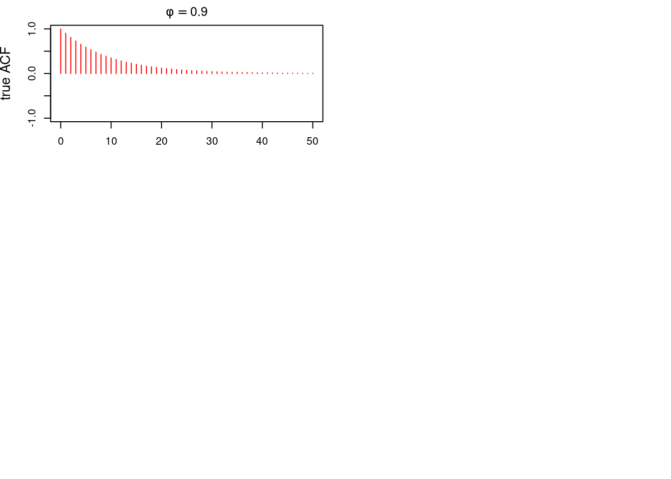
2. Exponential decay if $\|\phi\| < 1$
3. If $\phi > 0$: decay is monotonic
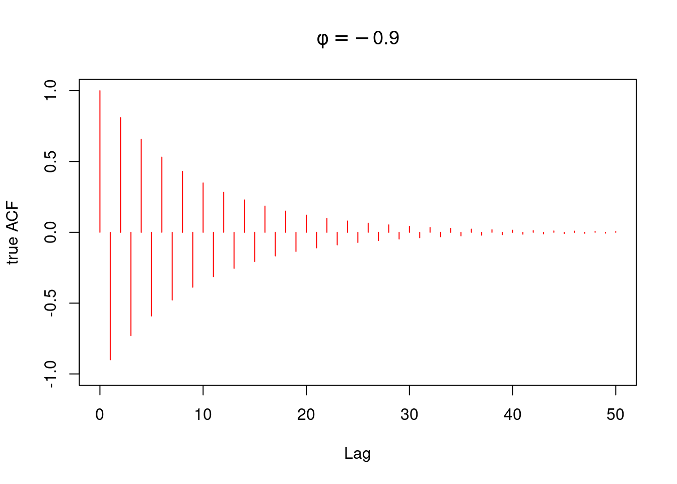
4. If $\phi < 0$: decay is **oscillatory** (alternates signs)
### Stationarity
\index{AR(1)!stationarity}
- The process is stationary when $\|\phi\| < 1$:
- Mean and variance are constant over time
- Autocovariance depends only on lag $h$, not on $t$
::: {.callout-note collapse="true"}
## Video Transcript
{{< include transcripts/c4/01_week-1-introduction-to-time-series-and-the-ar-1-process/03_the-ar-1-process-definition-and-properties/01_the-ar-1.en.txt >}}
:::
## The PACF of the AR(1) process :spiral_notepad:
\index{AR(1)!PACF}
\index{Durbin-Levinson recursion}
It is possible to show that the **PACF** of an *AR(1)* process is zero after the first lag.
We can use the **Durbin-Levinson recursion** to show this.
For lag $n = 0$ we have $\phi(0, 0) = 0$
For lag $n = 1$ we have:
$$
\phi(1, 1) = \rho(1) = \phi
$$ {#eq-ar1-pacf-lag1}
For lag $n = 2$ we compute $\phi(2, 2)$ as:
$$
\begin{aligned}
\phi(2, 2) &= \frac{(\rho(2) − \phi(1, 1)\rho(1))}{ (1 − \phi(1, 1)\rho(1))} \\
&= \frac{\phi^2-\phi^2}{1- \phi^2}\\
&=0
\end{aligned}
$$ {#eq-ar1-pacf-lag2}
and we also obtain:
$$
\phi(2, 1) = \phi(1, 1) − \phi(2, 2)\phi(1, 1) = \phi.
$$ {#eq-ar1-pacf-lag2-1}
For lag $n = 3$ we compute $\phi(3, 3)$ as
$$
\begin{aligned}
\phi(3, 3) &= \frac{(\rho(3) − \sum_{h=1}^2 \phi(2, h)\rho(3 − h))}{1 − \sum_{h=1}^2 \phi(2, h)\rho(h)} \newline
&= \frac{\phi^3 - \phi(2,1) \rho(2) - \phi(2,2) \rho(1)}{1 - \phi(2,1)\rho(1) - \phi(2,2)\rho(2)} \newline
&= \frac{\phi^3 - \phi^3 - 0}{1 - \phi^2 } \newline
&= 0
\end{aligned}
$$ {#eq-ar1-pacf-lag3}
and we also obtain
$$
\phi(3, 1) = \phi(2, 1) − \phi(3, 3)\phi(2, 2) = \phi
$$ {#eq-ar1-pacf-lag3-1}
$$
\phi(3, 2) = \phi(2, 2) − \phi(3, 3)\phi(2, 1) = 0
$$ {#eq-ar1-pacf-lag3-2}
We can prove by *induction* that in the case of an *AR(1)*, for any lag $n$,
$\phi(n, h) = 0, \phi(n, 1) = \phi$ and $\phi(n, h) = 0$ for $h \ge 2$ and $n \ge 2$.
Then, [the PACF of an AR(1) is zero for any lag above 1 and the **PACF** coefficient at lag 1 is equal to the AR coefficient $\phi$]{.mark}
## Simulate data from an AR(1) process :movie_camera: {#sec-ar1-simulation}
This video walks through the code snippet below and provides examples of how to sample data from an *AR(1)* process and plot the ACF and PACF functions of the resulting time series.
Prado demonstrates how to simulate *AR(1)* processes using `arima.sim` in R:
* **Simulation Setup**:
* `set.seed()` ensures reproducibility.
* Simulate 500 time points from an AR(1) with $\phi = 0.9$ and variance = 1.
* The process is stationary since $|\phi| < 1$.
* **arima.sim Function**:
* Can simulate ARIMA(p,d,q) processes; here, only AR(1) is used.
* Model specified via a list: `list(ar = phi)`, with `sd` as the standard deviation (√variance).
* **Comparative Simulation**:
* Second *AR(1)* simulated with $\phi = –0.9$ to show the impact of negative $\phi$.
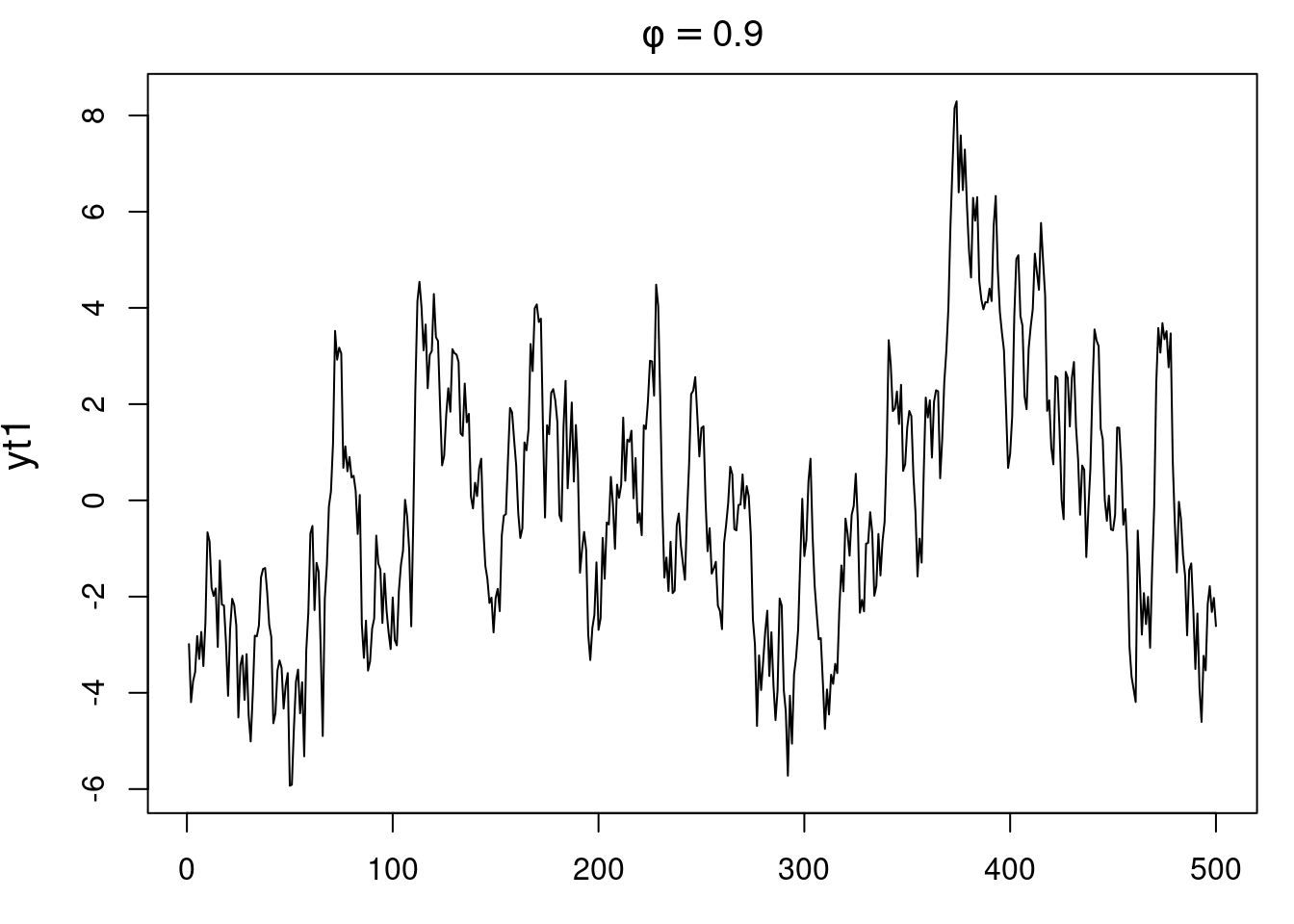
* The positive $\phi$ process shows persistent values (random walk-like).
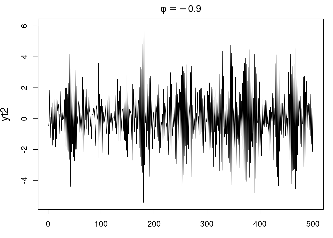
* The negative $\phi$ process shows oscillatory behavior.
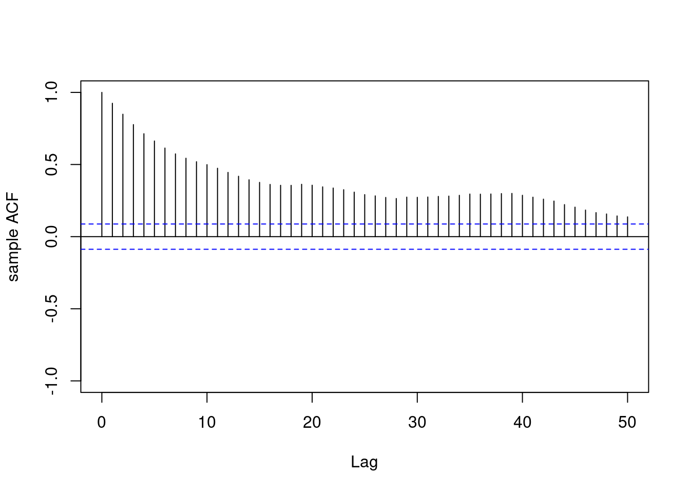
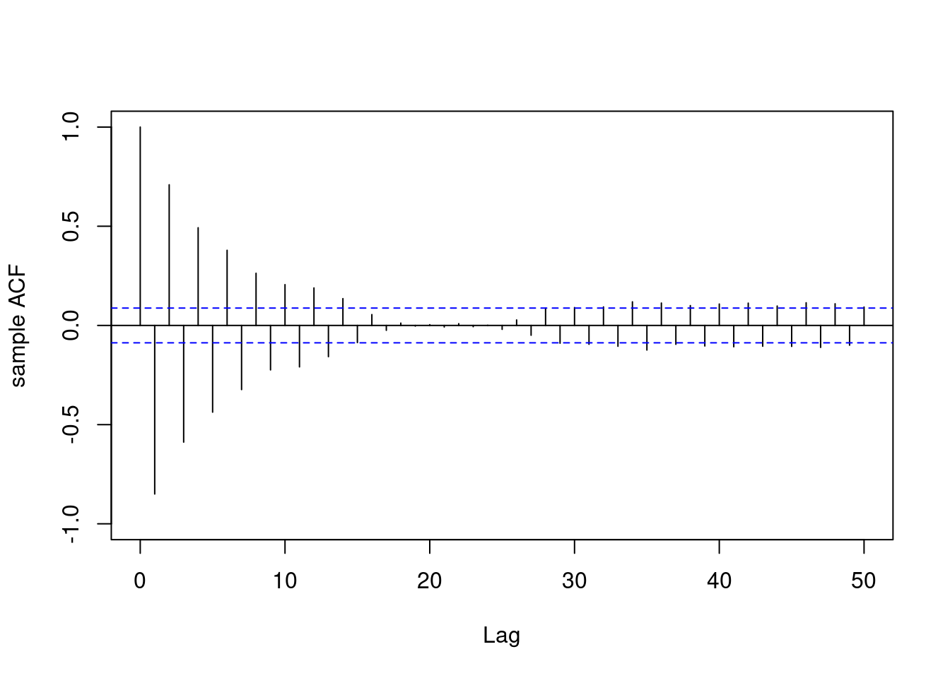
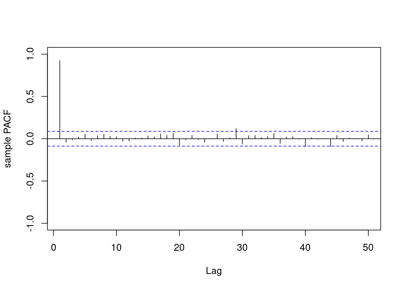
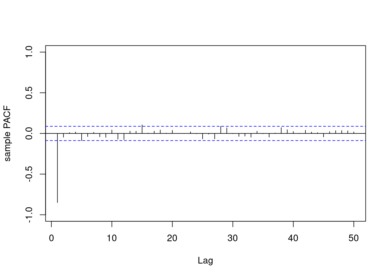
* **ACF and PACF Analysis**:
* **True ACF**: Exponential decay for both cases, oscillatory when $\phi < 0$.
* **Sample ACF**: Matches theoretical ACF for each process.
* **Sample PACF**: Only lag 1 is non-negligible, aligning with AR(1) properties:
* Positive at lag 1 for $\phi = 0.9$.
* Negative at lag 1 for $\phi = –0.9$.
* All other lags $≈ 0$.
The demonstration confirms our theoretical results regarding ACF/PACF behavior in AR(1) processes.
::: {.callout-note collapse="true"}
## Video Transcript
{{< include transcripts/c4/01_week-1-introduction-to-time-series-and-the-ar-1-process/03_the-ar-1-process-definition-and-properties/03_simulating-from-an-ar-1-process.en.txt >}}
:::
### R code: Sample data from AR(1) processes :spiral_notepad:
\index{AR(1)}
\index{AR(1)!ACF}
\index{AR(1)!PACF}
\index{ARIMA}
[Sample data from 2 ar(1) processes]{#l2g2 .mark}: and plot their ACF and PACF functions
```{r}
#| label: lst-ar1-sampling
set.seed(2021) # <1>
T=500 # <2>
v=1.0 # <3>
sd=sqrt(v) # <4>
phi1=0.9 # <5>
yt1=arima.sim( # <6>
n = T,
model = list(ar = phi1),
sd = sd) # <6>
phi2=-0.9 # <7>
yt2=arima.sim( # <8>
n = T,
model = list(ar = phi2),
sd = sd) # <8>
```
1. set seed for reproducibility
2. number of time points
3. innovation variance
4. innovation standard deviation
5. AR coefficient for the first process
6. Sample data from an **AR(1)** with coefficients $\phi = 0.9$ and $\nu = 1$
7. AR coefficient for the second process
8. Sample data from an **AR(1)** with coefficients $\phi = -0.9$ and $\nu = 1$
### Plot the time series of both processes
```{r}
#| label: fig-ar1-simulated
#| fig-cap: "Simulated AR(1) processes"
#| fig-subcap:
#| - $\phi = 0.9$
#| - $\phi = -0.9$
par(mfrow = c(1, 1),mar = c(3, 4, 2, 1), cex.lab = 1.3)
plot(yt1,main=expression(phi==0.9))
par(mfrow = c(1, 1),mar = c(3, 4, 2, 1), cex.lab = 1.3)
plot(yt2,main=expression(phi==-0.9))
```
### Plot true ACFs for both processes
```{r}
#| label: fig-acfs
#| fig-cap: "True ACF for the first AR(1) process"
par(mfrow = c(3, 2),mar = c(3, 4, 2, 1), cex.lab = 1.3)
lag.max=50 # max lag
cov_0=sd^2/(1-phi1^2) # <1>
cov_h=phi1^(0:lag.max)*cov_0 # <2>
plot(0:lag.max, cov_h/cov_0, pch = 1,
type = 'h', col = 'red',
ylab = "true ACF",
xlab = "Lag",
ylim=c(-1,1),
main=expression(phi==0.9)) # <3>
```
1. compute auto-covariance at h=0
2. compute auto-covariance at lag h
3. Plot autocorrelation function (ACF) for the first process
```{r}
#| label: fig-acfs2
#| fig-cap: "True ACF for the second AR(1) process"
cov_0=sd^2/(1-phi2^2) # <4>
cov_h=phi2^(0:lag.max)*cov_0 # <5>
# Plot autocorrelation function (ACF)
plot(0:lag.max, cov_h/cov_0, pch = 1,
type = 'h', col = 'red',
ylab = "true ACF",
xlab = "Lag",
ylim=c(-1,1),
main=expression(phi==-0.9)) # <6>
```
4. compute auto-covariance at h=0 for the second process
5. compute auto-covariance at lag h for the second process
6. Plot autocorrelation function (ACF) for the second process
### plot sample ACFs for both processes
```{r}
#| label: fig-sample-acfs
#| fig-cap: "Sample ACF for the first AR(1) process"
acf(yt1, lag.max = lag.max, type = "correlation", ylab = "sample ACF",
    lty = 1, ylim = c(-1, 1), main = " ")
acf(yt2, lag.max = lag.max, type = "correlation", ylab = "sample ACF",
    lty = 1, ylim = c(-1, 1), main = " ")
## plot sample PACFs for both processes

pacf(yt1, lag.ma = lag.max, ylab = "sample PACF", ylim=c(-1,1),main="")
pacf(yt2, lag.ma = lag.max, ylab = "sample PACF", ylim=c(-1,1),main="")
```