---
title : 'Computational Considerations - M5L8'
subtitle : 'Bayesian Statistics: Mixture Models'
categories:
- Bayesian Statistics
keywords:
- Mixture Models
- Maximum Likelihood Estimation
- BIC
- Bayesian Information Criteria
- Multimodality
- Numerical Instability
- notes
---
## Computational Considerations :movie_camera:
{#fig-s01-numerical-stability .column-margin width="53mm"}
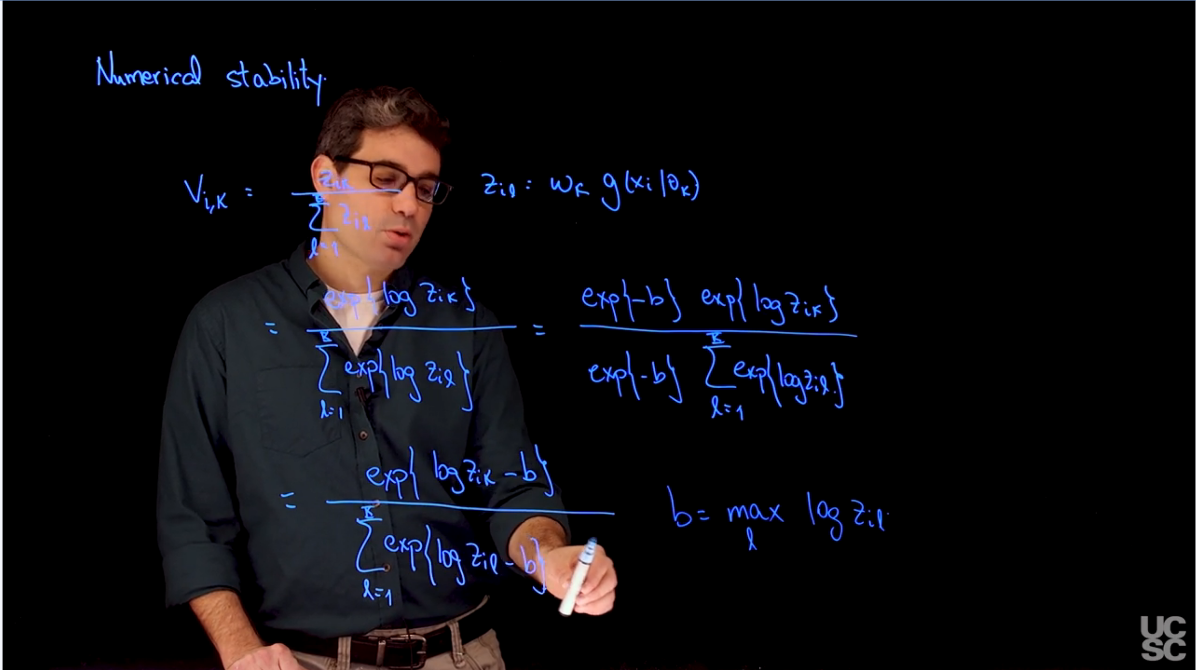
### Numerical stability
\index{mixture!Numerical stability}
\index{numerical stability}
The issue is in how the computer represents numbers. The computer uses a finite number of bits to represent numbers, which can lead to numerical instability when performing calculations that involve very large or very small numbers. This can result in loss of precision and incorrect results.
\index{transformations, logarithmic}
The solution is to use **logarithmic transformations** to avoid numerical instability. By taking the logarithm of the numbers, we can work with smaller and more manageable values, which reduces the risk of numerical instability.
### Sample code to illustrate numerical stability issues :spiral_notepad:
```{r}
#| label: lst-numeric-stability-sample-code
## Consider a mixture of two normal distributions with equal weights (w1 = w2 = 1/2)
## Component 1 has mean 0 and standard deviation 1
## Component 2 has mean 1 and standard deviation 1
## The observation is x = 50
## What is Pr(c = 1 | x)?
dnorm(50, 0, 1)
dnorm(50, 1, 1)
dnorm(50, 0, 1)/(dnorm(50, 0, 1) + dnorm(50, 1, 1))
## What if x=3?  Two ways to do the calculation
## One way:  Direct calculation
z1 = dnorm(3, 0, 1)
z2 = dnorm(3, 1, 1)
z1/(z1+z2)
## A second way:  Compute in the logarithm scale, add b
## to all values, and then exponentiate before standardizing
lz1 = dnorm(3, 0, 1, log=T)
lz2 = dnorm(3, 1, 1, log=T)
b = 3
exp(lz1+b)/(exp(lz1+b) + exp(lz2+b))
## Going back to the case x - 50:
## Wrong
lz1 = log(dnorm(50, 0, 1))
lz2 = log(dnorm(50, 1, 1))
b = max(lz1, lz2)
exp(lz1-b)/(exp(lz1-b) + exp(lz2-b))
## Wrong
lz1 = log(exp(-0.5*50^2)/sqrt(2*pi))
lz2 = log(exp(-0.5*49^2)/sqrt(2*pi))
b = max(lz1, lz2)
exp(lz1-b)/(exp(lz1-b) + exp(lz2-b))
## Right
lz1 = dnorm(50, 0, 1, log=TRUE)
lz2 = dnorm(50, 1, 1, log=TRUE)
b = max(lz1, lz2)
exp(lz1-b)/(exp(lz1-b) + exp(lz2-b))
## Also right (just more cumbersome)
lz1 = -0.5*log(2*pi) - 0.5*50^2
lz2 = -0.5*log(2*pi) - 0.5*49^2
b = max(lz1, lz2)
exp(lz1-b)/(exp(lz1-b) + exp(lz2-b))
```
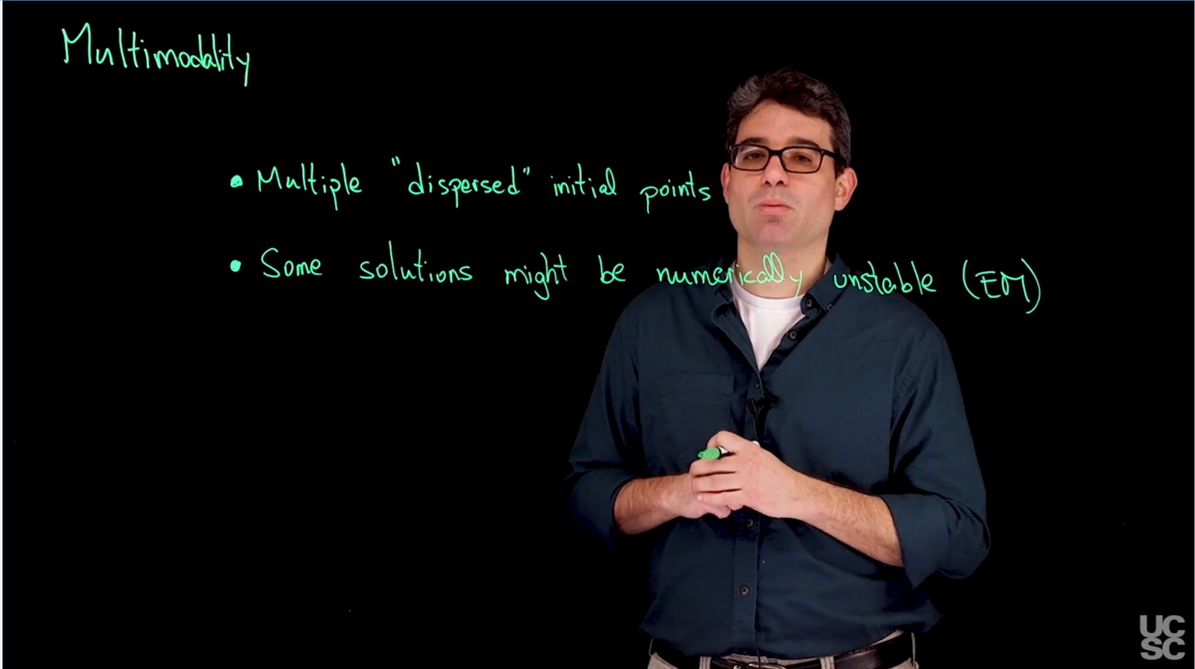
### Computational issues associated with multimodality :movie_camera: {#sec-computational-issues}
{#fig-s02-multimodality .column-margin width="53mm"}
### Sample code to illustrate multimodality issues 1 :spiral_notepad: {#sec-multimodality-1}
\index{dataset!iris}
\index{multimodality}
\index{numerical instability}
```{r}
#| label: lst-multimodality-sample-code-1
## Illustrating the fact that the likelihood for a mixture model is multimodal

### Loading data and setting up global variables
rm(list=ls())
library(mclust)
library(mvtnorm)
### Defining a custom function to create pair plots
### This is an alternative to the R function pairs() that allows for
### more flexibility. In particular, it allows us to use text to label
### the points
pairs2 = function(x, col="black", pch=16, labels=NULL, names = colnames(x)){
  n = dim(x)[1]
  p = dim(x)[2]
  par(mfrow=c(p,p))
  for(k in 1:p){
    for(l in 1:p){
      if(k!=l){
        par(mar=c(3,3,1,1)+0.1)
        plot(x[,k], x[,l], type="n", xlab="", ylab="")
        if(is.null(labels)){
          points(x[,k], x[,l], pch=pch, col=col)
        }else{
          text(x[,k], x[,l], labels=labels, col=col)
        }
      }else{
        plot(seq(0,5), seq(0,5), type="n", xlab="", ylab="", axes=FALSE)
        text(2.5,2.5,names[k], cex=1.2)
      }
    }
  }
}


## Setup data
data(iris)
x       = as.matrix(iris[,-5])
n       = dim(x)[1]
p       = dim(x)[2]       # Number of features
KK      = 3
epsilon = 0.0000001
par(mfrow=c(1,1))
par(mar=c(4,4,1,1))
colscale = c("black","blue","red")
shortnam  = c("s","c","g")

# Initialize the parameters of the algorithm
set.seed(63252)

numruns = 15
v.sum   = array(0, dim=c(numruns, n, KK))
QQ.sum  = rep(0, numruns)

for(ss in 1:numruns){
  w   = rep(1,KK)/KK  #Assign equal weight to each component to start with
  #mu  = as.matrix(aggregate(x, list(iris[,5]), mean)[,2:5])  # Initialize in the true values
  #Sigma      = array(0, dim=c(KK,p,p))  #Initial variances are assumed to be the same
  #Sigma[1,,] = var(x[iris[,5]=="setosa",])
  #Sigma[2,,] = var(x[iris[,5]=="versicolor",])
  #Sigma[3,,] = var(x[iris[,5]=="virginica",])
  mu  = rmvnorm(KK, apply(x,2,mean), 3*var(x))   #Cluster centers randomly spread over the support of the data
  Sigma      = array(0, dim=c(KK,p,p))  #Initial variances are assumed to be the same
  Sigma[1,,] = var(x)
  Sigma[2,,] = var(x)
  Sigma[3,,] = var(x)

  sw     = FALSE
  QQ     = -Inf
  QQ.out = NULL
  s      = 0

  while(!sw){
    ## E step
    v = array(0, dim=c(n,KK))
    for(k in 1:KK){  #Compute the log of the weights
      v[,k] = log(w[k]) + dmvnorm(x, mu[k,], Sigma[k,,], log=TRUE)
    }
    for(i in 1:n){
      v[i,] = exp(v[i,] - max(v[i,]))/sum(exp(v[i,] - max(v[i,])))  #Go from logs to actual weights in a numerically stable manner
    }

    ## M step
    w = apply(v,2,mean)
    mu = matrix(0, nrow=KK, ncol=p)
    for(k in 1:KK){
      for(i in 1:n){
        mu[k,]    = mu[k,] + v[i,k]*x[i,]
      }
      mu[k,] = mu[k,]/sum(v[,k])
    }
    Sigma = array(0,dim=c(KK, p, p))
    for(k in 1:KK){
      for(i in 1:n){
        Sigma[k,,] = Sigma[k,,] + v[i,k]*(x[i,] - mu[k,])%*%t(x[i,] - mu[k,])
      }
      Sigma[k,,] = Sigma[k,,]/sum(v[,k])
    }

    ##Check convergence
    QQn = 0
    for(i in 1:n){
      for(k in 1:KK){
        QQn = QQn + v[i,k]*(log(w[k]) + dmvnorm(x[i,],mu[k,],Sigma[k,,],log=TRUE))
      }
    }
    if(abs(QQn-QQ)/abs(QQn)<epsilon){
      sw=TRUE
    }
    QQ = QQn
    QQ.out = c(QQ.out, QQ)
    s = s + 1
  }

  v.sum[ss,,] = v
  QQ.sum[ss]  = QQ.out[s]
  print(paste("ss =", ss))
}
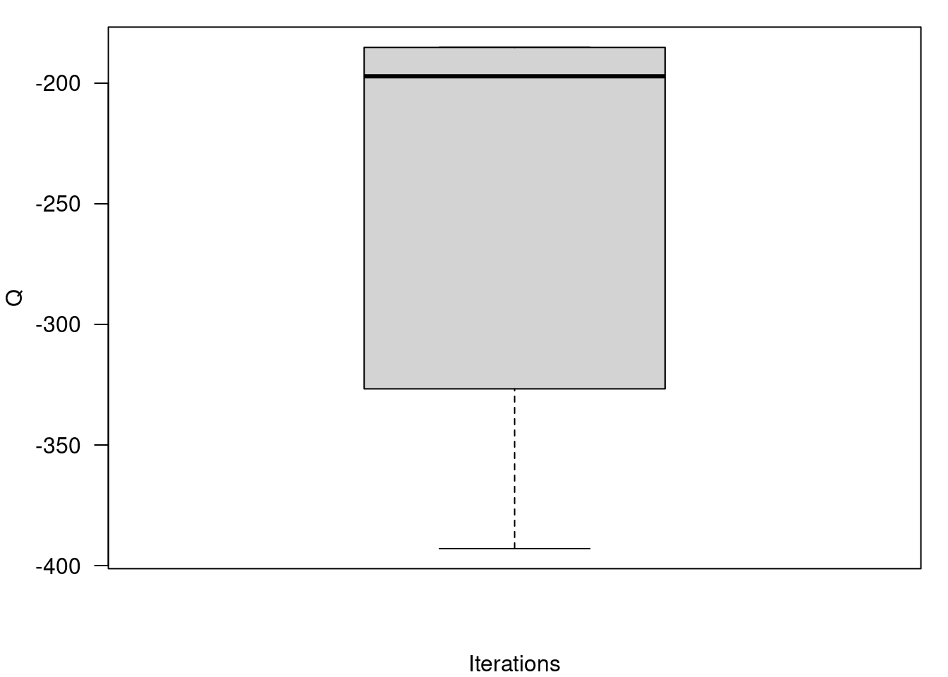
## Boxplot of final values of the Q function for all runs of the algorithm
par(mfrow=c(1,1))
par(mar=c(4,4,1,1))
boxplot(QQ.out, ylab="Q", xlab="Iterations",las=2)
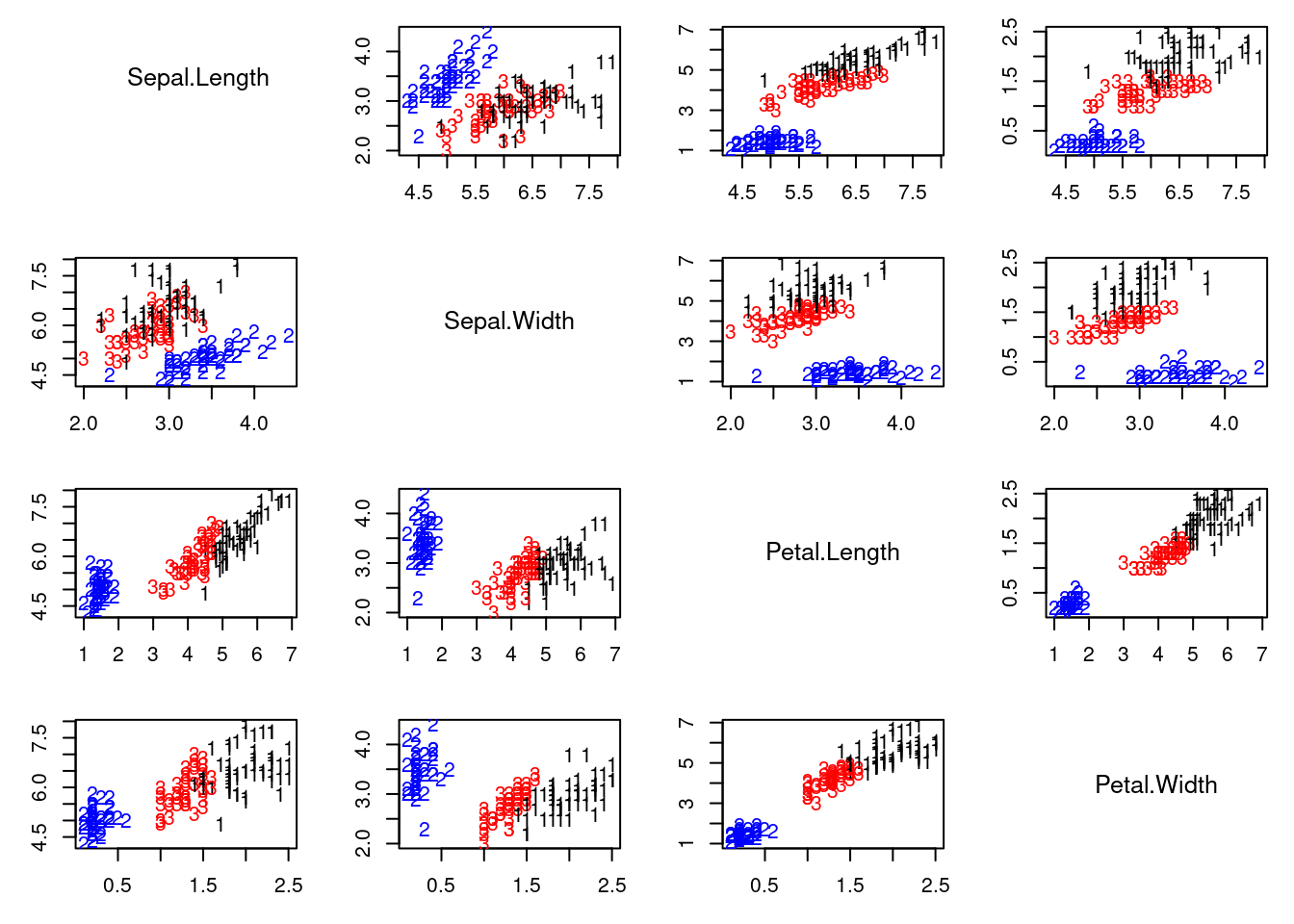
## Graphical representation of the best solution
cc = apply(v.sum[which.max(QQ.sum),,], 1 ,which.max)
colscale = c("black","blue","red")
#pairs(x, col=colscale[cc], pch=cc)
pairs2(x, col=colscale[cc], labels=cc)
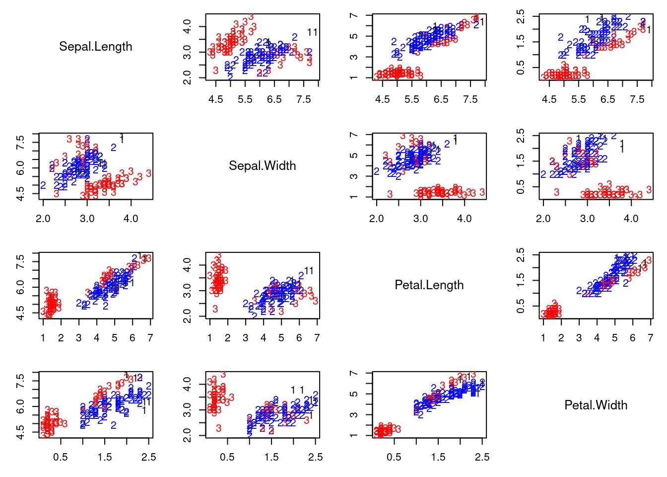
## Graphical representation of the worst solution
cc = apply(v.sum[which.min(QQ.sum),,], 1 ,which.max)
colscale = c("black","blue","red")
#pairs(x, col=colscale[cc], pch=cc)
pairs2(x, col=colscale[cc], labels=cc)
```
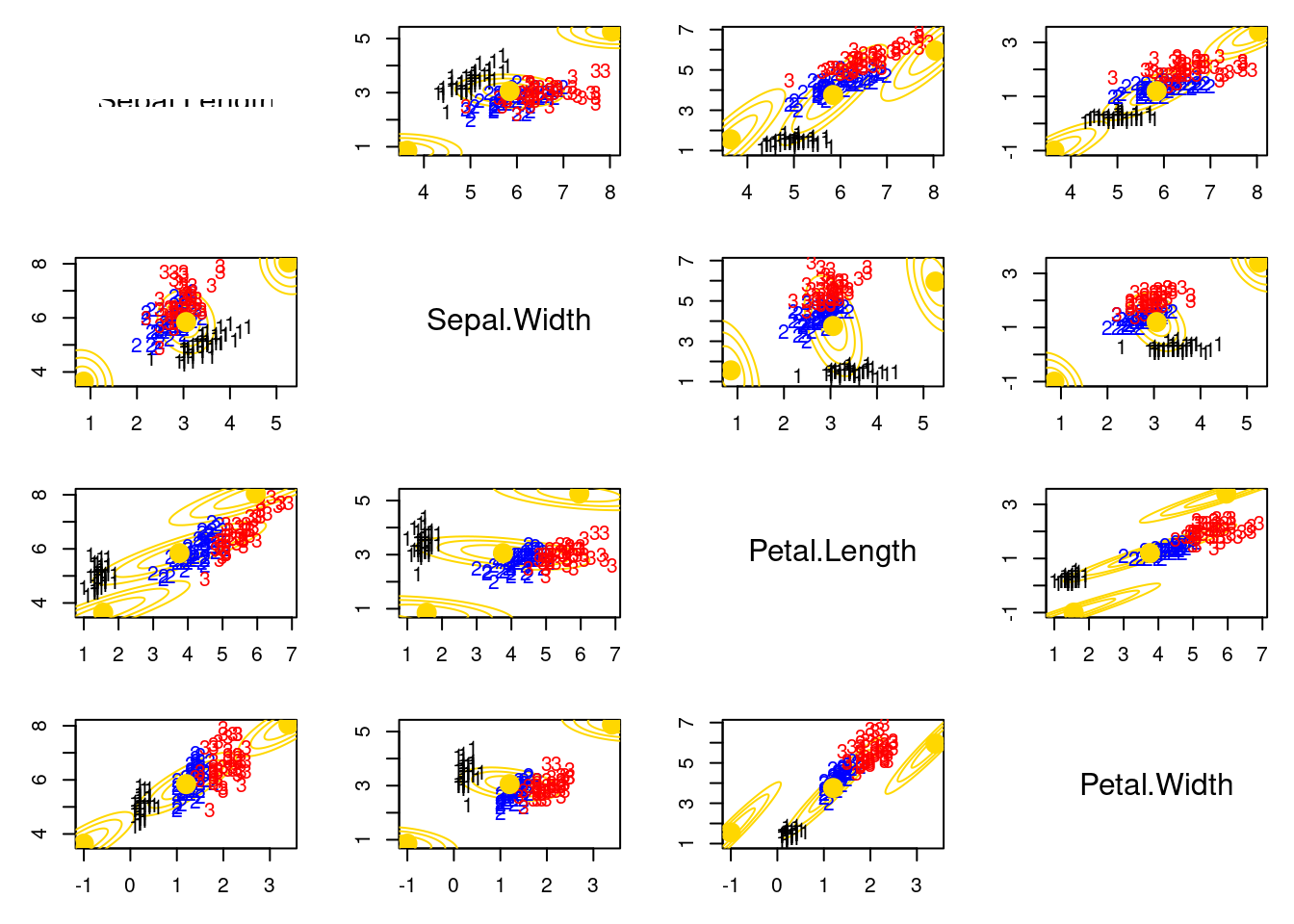
### Sample code to illustrate multimodality issues 2 :spiral_notepad: {#sec-multimodality-2}
This code fails to converge because the algorithm is stuck in a local maximum of the likelihood function. The problem is that one of the components is "numerically empty" (i.e., it has no data points assigned to it). [This can happen when the initial values for the means are too far apart or when the data is not well-separated.]{.mark}
```{r}
#| label: lst-multimodality-sample-code-2
#| error: true
## Illustrating that the EM might fail for numerical reasons if a component is “numerically empty”

### Loading data and setting up global variables
rm(list=ls())
library(mclust)
library(mvtnorm)
library(ellipse)
## Setup data
data(iris)
x       = as.matrix(iris[,-5])
n       = dim(x)[1]
p       = dim(x)[2]       # Number of features
KK      = 3
epsilon = 0.00000001

# Initialize the parameters of the algorithm
w   = rep(1,KK)/KK  #Assign equal weight to each component to start with
mu  = matrix(0, KK, p)  # Initialize in the true values
mu[1,] = apply(x, 2, mean)
mu[2,] = apply(x, 2, mean) + c(2.2, 2.2, 2.2, 2.2)
mu[3,] = apply(x, 2, mean) + c(-2.2, -2.2, -2.2, -2.2)
Sigma      = array(0, dim=c(KK,p,p))  #Initial variances are assumed to be the same
Sigma[1,,] = var(x)/3
Sigma[2,,] = var(x)/3
Sigma[3,,] = var(x)/3

# Plot the data along with the estimates of the components
colscale = c("black","blue","red")
par(mfrow=c(p,p))
for(k in 1:p){
  for(l in 1:p){
    if(k!=l){
      par(mar=c(3,3,1,1)+0.1)
      plot(x[,k], x[,l], type="n", xlab="", ylab="", xlim=c(min(c(x[,k], mu[,k])),max(c(x[,k], mu[,k]))), ylim=c(min(c(x[,l], mu[,l])),max(c(x[,l], mu[,l]))))
      for(r in 1:KK){
        lines(ellipse(x=Sigma[r,c(k,l),c(k,l)], centre=mu[r,c(k,l)], level=0.50), col="gold1", lty=1, lwd=1)
        lines(ellipse(x=Sigma[r,c(k,l),c(k,l)], centre=mu[r,c(k,l)], level=0.82), col="gold1", lty=1, lwd=1)
        lines(ellipse(x=Sigma[r,c(k,l),c(k,l)], centre=mu[r,c(k,l)], level=0.95), col="gold1", lty=1, lwd=1)
      }
      text(x[,k], x[,l], labels=as.numeric(iris[,5]), col=colscale[iris[,5]])
      points(mu[,k], mu[,l], pch=19, col="gold1", cex=2)
    }else{
      plot(seq(0,5), seq(0,5), type="n", xlab="", ylab="", axes=FALSE)
      text(2.5,2.5,colnames(x)[k], cex=1.5)
    }
  }
}
## Run the EM algorithm.  It will fail in the first iteration
sw     = FALSE
QQ     = -Inf
QQ.out = NULL
s      = 0

while(!sw){
  ## E step
  v = array(0, dim=c(n,KK))
  for(k in 1:KK){  #Compute the log of the weights
    v[,k] = log(w[k]) + dmvnorm(x, mu[k,], Sigma[k,,], log=TRUE)
  }
  for(i in 1:n){
    v[i,] = exp(v[i,] - max(v[i,]))/sum(exp(v[i,] - max(v[i,])))  #Go from logs to actual weights in a numerically stable manner
  }

  ## M step
  w = apply(v,2,mean)
  mu = matrix(0, nrow=KK, ncol=p)
  for(k in 1:KK){
    for(i in 1:n){
      mu[k,]    = mu[k,] + v[i,k]*x[i,]
    }
    mu[k,] = mu[k,]/sum(v[,k])
  }
  Sigma = array(0,dim=c(KK, p, p))
  for(k in 1:KK){
    for(i in 1:n){
      Sigma[k,,] = Sigma[k,,] + v[i,k]*(x[i,] - mu[k,])%*%t(x[i,] - mu[k,])
    }
    Sigma[k,,] = Sigma[k,,]/sum(v[,k])
  }

  ##Check convergence
  QQn = 0
  for(i in 1:n){
    for(k in 1:KK){
      QQn = QQn + v[i,k]*(log(w[k]) + dmvnorm(x[i,],mu[k,],Sigma[k,,],log=TRUE))
    }
  }
  if(abs(QQn-QQ)/abs(QQn)<epsilon){
    sw=TRUE
  }
  QQ = QQn
  QQ.out = c(QQ.out, QQ)
  s = s + 1
}
QQn
```