Appendix B — Appendix: Discrete Distributions

B.1 Discrete Uniform

B.1.1 Stories

NoteDiscrete Uniform Finite set Parametrization

Let C be a finite, nonempty set of numbers and X random variable associated with the event of choosing one of these numbers uniformly at random, that is all values being equally likely X(x=c)

Then X is said to have the Discrete Uniform distribution with parameter C.

We denote this by X ∼ DUnif(C).

NoteDiscrete Uniform with Lower and Upper bound Parametrization

When the set C above is C=\{c \in \mathbb{Z} \mid a \le c \le b\ \}.

Then X is said to have the Discrete Uniform distribution with lower bound parameter a and upper bound parameter b.

We denote this by X ∼ DUnif(a,b).

NoteUrn Model

Suppose we have an urn with n balls labeled with the numbers a 1, \dots, a_n . One drawing from the urn produces a discrete uniform random variable on the set \{a_1, \dots, a_n \}.

B.1.2 Moments

\begin{aligned} \phi_X(t)&={\displaystyle {\frac {e^{at}-e^{(b+1)t}}{n(1-e^{t})}}} && \text{(MGF)}\\ \mathbb{E}[X] &= \frac{a + b}{2} && \text{(Expectation)} \\ \mathbb{V}ar[X] &= \frac{(b - a + 1)^2 - 1}{12} && \text{(Variance)} \end{aligned} \tag{B.1}

B.1.3 Probability mass function (PMF)

f(x \mid a, b) = \frac{1}{b - a + 1}

B.1.4 Cumulative distribution function (CDF)

F(x \mid a, b) = \frac{\lfloor x \rfloor - a - 1}{b - a + 1} \\ \text{where} \lfloor x \rfloor \text{ is the floor function (rounds down reals to nearest smaller integer)}

B.1.5 Prior

Since a number of families have the uniform as a special case we can use them as priors when we want a uniform prior:

B.2 Bernoulli Distribution

.

B.2.1 Stories

Note

The Bernoulli distribution arises when modeling the outcome of a binary event called a Bernoulli trial.

Let X be the indicator variable corresponding to the success of getting “heads” in a “coin toss”, with a coin that has probability of success p for getting “heads”.

Then X has a Bernoulli Distribution with parameter p

We denote this as X \sim Bern(p)

B.2.2 Parameters

Because of this story, the parameter p is often called the success probability of the Bern(p) distribution.

B.2.3 Examples

Note

• fair coin toss
• unfair coin toss
• ad click
• web site conversion
• death or survival of a patient in a medical trial
• indicator random variable

B.2.4 Checklist

Note

• Discrete data
• A single trial
• Only two trial outcomes: success and failure (These do not need to literally represent successes and failures, but this shorthand is typically used.)

\begin{aligned} X &\sim Bernoulli(p)\\ & \sim Bern(p)\\ & \sim B(p) \end{aligned} \tag{B.2}

B.2.5 Moments

M_X(t)=q+pe^{t} \qquad \text{(MGF)} \tag{B.3}

\mathbb{E}[X]= p \qquad \text{(Expectation)} \tag{B.4}

\mathbb{V}ar[x]= \mathbb{P}r(1-p) \qquad \text{(Variance)} \tag{B.5}

B.2.6 PMF

Where parameter p is the probability of getting heads.

The probability for the two events is:

\mathbb{P}r(X=1) = p \qquad \mathbb{P}r(X=0)=1-p

\begin{cases} 1-p & \text{if } k=0 \\ p & \text{if } k=1 \end{cases} \qquad \text{(PMF)} \tag{B.6}

B.2.7 CDF

\begin{cases} 0&{\text{if }}k<0 \\ 1-p&{\text{if }}0\leq k<1 \\ 1&{\text{if }}k\geq 1 \end{cases} \qquad \text{(CDF)} \tag{B.7}

B.2.8 Likelihood

L(\theta) = \prod p^x(1-p)^{1-x} \mathbb{I}_{[0,1]}(x) \qquad \text{(Likelihood)} \tag{B.8}

\mathcal{L}(\theta) =log(p) \sum x + log(1-p)\sum (1-x) \qquad \text{(Log Likelihood)} \tag{B.9}

B.2.9 Entropy and Information

\mathbb{H}(x)= -q \ln(q)- p \ln(p) \qquad \text{(Entropy)} \tag{B.10}

\mathcal{I}[X]\frac{1}{\mathbb{P}r(1-p)} \qquad \text{(Fisher Information)} \tag{B.11}

Beta(x) \qquad \text{(Conjugate Prior)} \tag{B.12}

B.2.10 Usage

Table B.1: Usage of Bernoulli

Package	Syntax
NumPy	rg.choice([0, 1], p=[1-theta, theta])
SciPy	scipy.stats.bernoulli(theta)
Stan	bernoulli(theta)

B.2.11 Plots

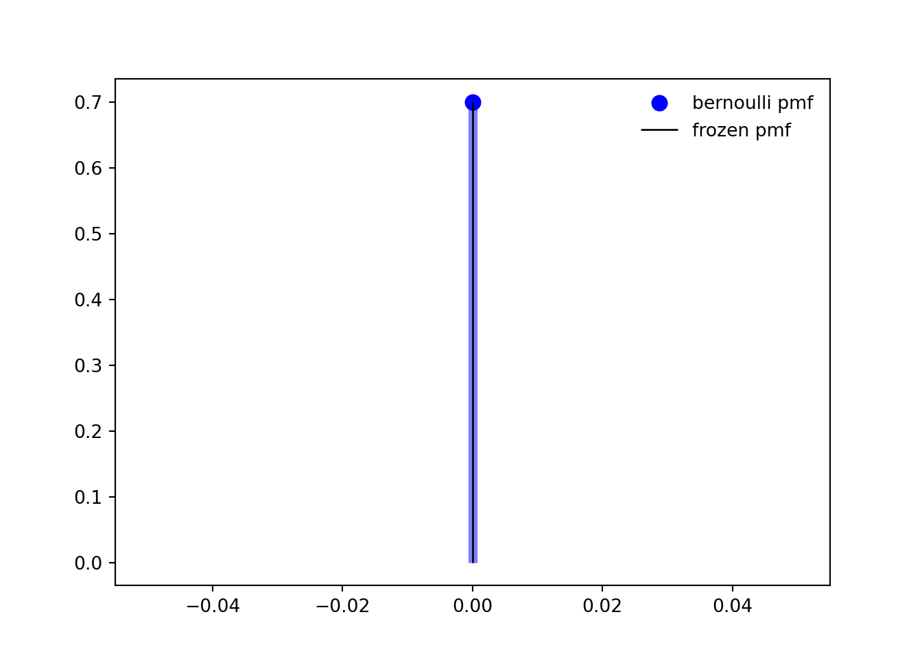
import numpy as np
from scipy.stats import bernoulli
import matplotlib.pyplot as plt

fig, ax = plt.subplots(1, 1)
p = 0.3
mean, var, skew, kurt = bernoulli.stats(p, moments='mvsk')
print(f'{mean=:1.2f}, {var=:1.2f}, {skew=:1.2f}, {kurt=:1.2f}')

mean=0.30, var=0.21, skew=0.87, kurt=-1.24

x = np.arange(bernoulli.ppf(0.01, p),
              bernoulli.ppf(0.99, p))
ax.plot(x, bernoulli.pmf(x, p), 'bo', ms=8, label='bernoulli pmf')
ax.vlines(x, 0, bernoulli.pmf(x, p), colors='b', lw=5, alpha=0.5)

rv = bernoulli(p)
ax.vlines(x, 0, rv.pmf(x), colors='k', linestyles='-', lw=1,
        label='frozen pmf')
ax.legend(loc='best', frameon=False)
plt.show()

## Generate random numbers
r = bernoulli.rvs(p, size=10)
r

array([0, 0, 0, 0, 1, 1, 1, 0, 0, 0])

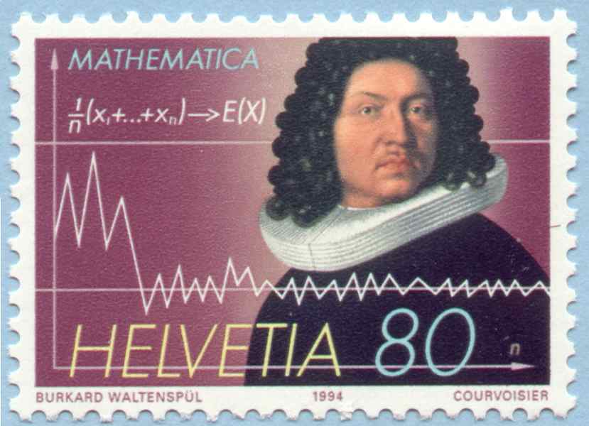
A Swiss stamp issueed in 1994 depicting Mathematician Jakob Bernouilli and the formula and diagram of the law of large numbers

TipBiographical note on Jacob Bernoulli

It seems that to make a correct conjecture about any event whatever, it is necessary to calculate exactly the number of possible cases and then to determine how much more likely it is that one case will occur than another. (Bernoulli 1713)

The Bernoulli distribution as well as The Binomial distribution are due to Jacob Bernoulli (1655-1705) who was a prominent mathematician in the Bernoulli family. He discovered the fundamental mathematical constant e. With his brother Johann, he was among the first to develop Leibniz’s calculus, introducing the word integral and applying it to polar coordinates and the study of curves such as the catenary, the logarithmic spiral and the cycloid

His most important contribution was in the field of probability, where he derived the first version of the law of large numbers (LLN). The LLN is a theorem that describes the result of performing the same experiment a large number of times. According to the law, the average of the results obtained from a large number of trials should be close to the expected value and will tend to become closer to the expected value as more trials are performed. A special form of the LLN (for a binary random variable) was first proved by Jacob Bernoulli. It took him over 20 years to develop sufficiently rigorous mathematical proof.

For a more extensive biography visit the following link

The Bernoulli distribution is built on a trial of a coin toss (possibly biased).

• We use the Bernoulli distribution to model a random variable for the probability of such a coin toss trial.
• We use the Binomial distribution to model a random variable for the probability of getting k heads in N independent trails.

B.3 Binomial distribution

B.3.1 Stories

Note

\overbrace{\underbrace{\fbox{0}\ \ldots \fbox{0}}_{N_0}\ \underbrace{\fbox{1}\ \ldots \fbox{1}}_{N_1}}^N \tag{B.13}

The Binomial distribution arises when we conduct multiple independent Bernoulli trials and wish to model X the number of successes in Y_i\mid \theta identically distributed Bernoulli trials with the same probability of success \theta. If n independent Bernoulli trials are performed, each with the same success probability p. The distribution of X is called the Binomial distribution with parameters n and p. We write X \sim \text{Bin}(n, p) to mean that X has the Binomial distribution with parameters n and p, where n is a positive integer and 0 < p < 1.

B.3.2 Parameters

• \theta - the probability of success in the Bernoulli trials
• N - the total number of trials being conducted

B.3.3 Conditions

Tip

• Discrete data
• Two possible outcomes for each trial
• Each trial is independent and
• The probability of success/failure is the same in each trial
• The outcome is the aggregate number of successes

B.3.4 Examples

• to model the aggregate outcome of clinical drug trials,
• to estimate the proportion of the population voting for each political party using exit poll data (where there are only two political parties).

X \sim Bin[n,p] \tag{B.14}

f(X=x \mid \theta) = {n \choose x} \theta^x(1-\theta)^{n-x} \tag{B.15}

L(\theta)=\prod_{i=1}^{n} {n\choose x_i} \theta ^ {x_i} (1− \theta) ^ {(n−x_i)} \tag{B.16}

\begin{aligned} \ell( \theta) &= \log \mathcal{L}( \theta) \\ &= \sum_{i=1}^n \left[\log {n\choose x_i} + x_i \log \theta + (n-x_i)\log (1- \theta) \right] \end{aligned} \tag{B.17}

\mathbb{E}[X]= N \times \theta \tag{B.18}

\mathbb{V}ar[X]=N \cdot \theta \cdot (1-\theta) \tag{B.19}

\mathbb{H}(X) = \frac{1}{2}\log_2 \left (2\pi n \theta(1 - \theta)\right) + O(\frac{1}{n}) \tag{B.20}

\mathcal{I}(\theta)=\frac{n}{ \theta \cdot (1- \theta)} \tag{B.21}

B.3.5 Usage

Table B.2: Usage of Binomial

Package	Syntax
NumPy	rg.binomial(N, theta)
SciPy	scipy.stats.binom(N, theta)
Stan	binomial(N, theta)

B.3.6 Relationships

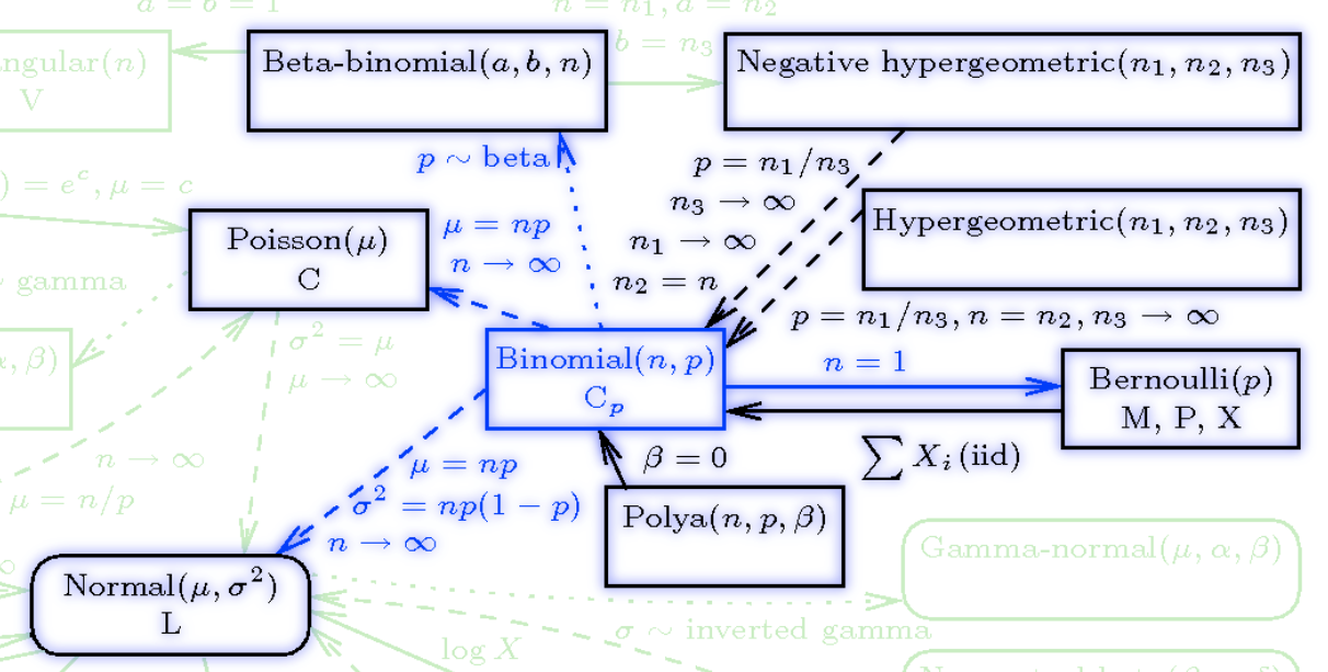
binomial distribution relations

The Binomial Distribution is related to

• The Binomial is a special case of the Multinomial distribution with K =2 (two categories).
• the Poisson distribution distribution. If X \sim Binomial(n, p) rv and Y \sim Poisson(np) distribution then \mathbb{P}r(X = n) ≈ \mathbb{P}r(Y = n) for large n and small np.
• The Bernoulli distribution is a special case of the the Binomial distribution \begin{aligned} X & \sim \mathrm{Binomial}(n=1, p) \\ \implies X &\sim \mathrm{Bernoulli}(p) \end{aligned}
• the Normal distribution If X \sim \mathrm{Binomial}(n, p) RV and Y \sim \mathcal{N}(\mu=np,\sigma=n\mathbb{P}r(1-p)) then for integers j and k, \mathbb{P}r(j ≤ X ≤ k) ≈ \mathbb{P}r(j – 1/2 ≤ Y ≤ k + 1/2). The approximation is better when p ≈ 0.5 and when n is large. For more information, see normal approximation to the Binomial
• The Binomial is a limit of the Hypergeometric. The difference between a binomial distribution and a hypergeometric distribution is the difference between sampling with replacement and sampling without replacement. As the population size increases relative to the sample size, the difference becomes negligible. So If X \sim \mathrm{Binomial}(n, p) RV and Y \sim \mathrm{HyperGeometric}(N,a,b) then

\lim_{n\to \infty} X = Y

B.3.7 Plots

import numpy as np
from scipy.stats import binom
import matplotlib.pyplot as plt
fig, ax = plt.subplots(1, 1)
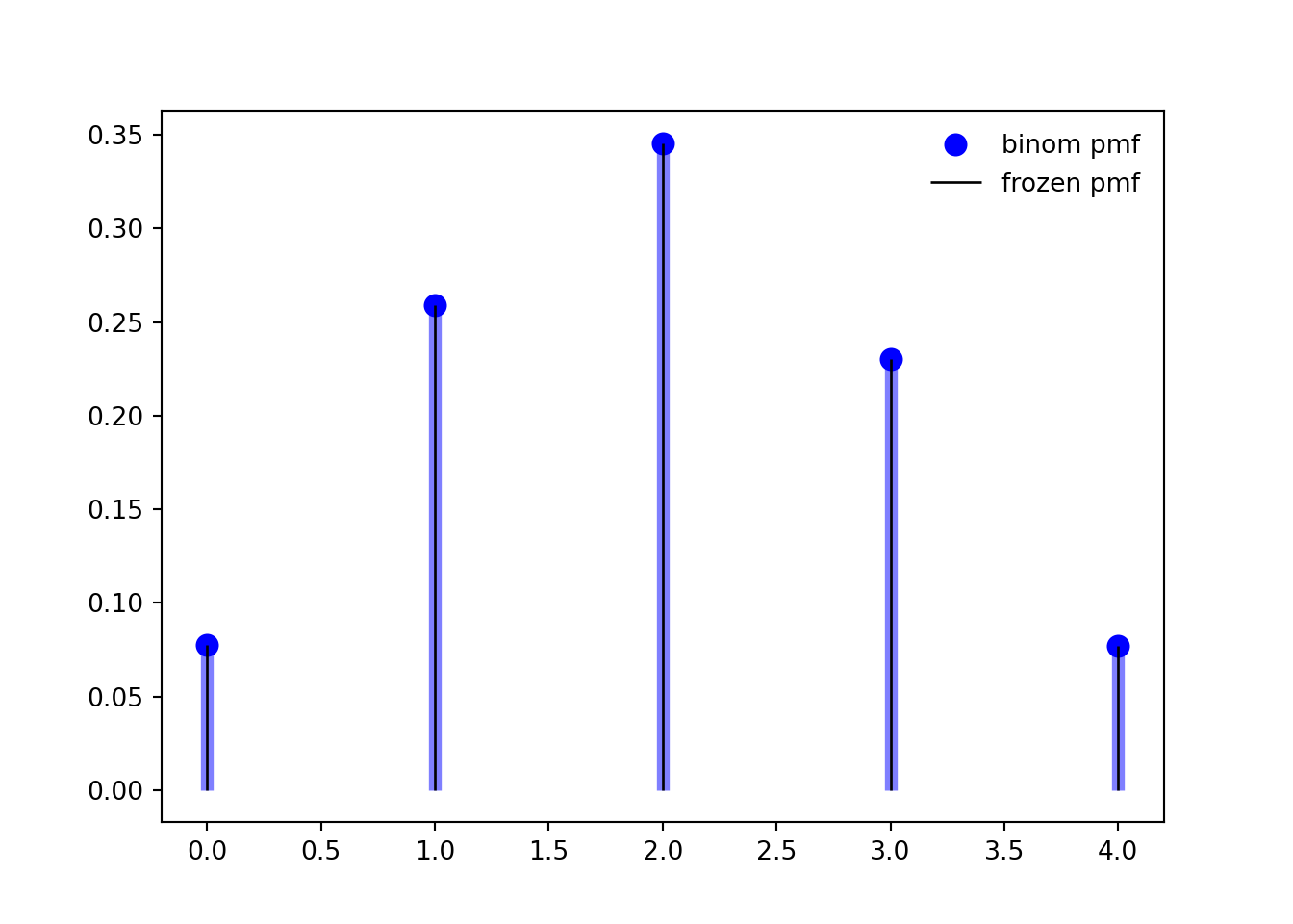
n, p = 5, 0.4
mean, var, skew, kurt = binom.stats(n, p, moments='mvsk')
print(f'{mean=:1.2f}, {var=:1.2f}, {skew=:1.2f}, {kurt=:1.2f}')

mean=2.00, var=1.20, skew=0.18, kurt=-0.37

x = np.arange(binom.ppf(0.01, n, p),
              binom.ppf(0.99, n, p))
ax.plot(x, binom.pmf(x, n, p), 'bo', ms=8, label='binom pmf')
ax.vlines(x, 0, binom.pmf(x, n, p), colors='b', lw=5, alpha=0.5)
rv = binom(n, p)
ax.vlines(x, 0, rv.pmf(x), colors='k', linestyles='-', lw=1,
        label='frozen pmf')
ax.legend(loc='best', frameon=False)
plt.show()

## generate random numbers
r = binom.rvs(n, p, size=10)
r

array([2, 1, 2, 4, 4, 1, 3, 1, 3, 2])

from __future__ import print_function
from ipywidgets import interact, interactive, fixed, interact_manual
import ipywidgets as widgets
import numpy as np
import scipy
from scipy.special import gamma, factorial, comb
import plotly.express as px
import plotly.offline as pyo
import plotly.graph_objs as go
#pyo.init_notebook_mode()
INTERACT_FLAG=False
def binomial_vector_over_y(theta, n):
    total_events = n
    y =  np.linspace(0, total_events , total_events + 1)
    p_y = [comb(int(total_events), int(yelem)) * theta** yelem * (1 - theta)**(total_events - yelem) for yelem in y]

    fig = px.line(x=y, y=p_y, color_discrete_sequence=["steelblue"], 
                  height=600, width=800, title=" Binomial distribution for theta = %lf, n = %d" %(theta, n))
    fig.data[0].line['width'] = 4
    fig.layout.xaxis.title.text = "y"
    fig.layout.yaxis.title.text = "P(y)"
    fig.show()
    
if(INTERACT_FLAG):    
    interact(binomial_vector_over_y, theta=0.5, n=15)
else:
    binomial_vector_over_y(theta=0.5, n=10)

Video B.1: Binomial Distribution

B.4 Hypergeometric distribution

B.4.1 story 1 - Urn Model

The beta-binomial distribution with parameters \alpha success rate and \beta failure and n the number of trials can be motivated by an Pólya urn model.

Imagine a trial in which a ball is drawn without replacement from urn containing \alpha white balls and \beta black balls. If this is repeated n times, then the probability of observing x white balls follows a hypergeometric distribution with parameters n, \alpha and \beta.

Note: is we used a

If the random draws are with simple replacement (no balls over and above the observed ball are added to the urn), then the distribution follows a binomial distribution and if the random draws are made without replacement, the distribution follows a hypergeometric distribution.

Video B.2: The Hypergeometric Distribution

B.4.2 Examples

• k white balls from an in Urn without replacement
• capture-recapture
• Aces in a poker hand

B.4.3 Story

Consider an urn with w white balls and b black balls. We draw n balls out of the urn at random without replacement, such that all w+b samples are equally likely. Let X be the number of white balls in n the sample. Then X is said to have the Hypergeometric distribution with parameters w, b, and n; we denote this by X \sim \mathcal{HG}(w, b, n) or X \sim \mathrm{HyperGeom}(w, b, n) or

B.5 Poisson distribution

B.5.1 Stories

NotePoisson Parametrization

The Poisson distribution arises when modeling the number of successes of independent and identically distributed (IID) events in a fixed interval of time or space, occurring at a constant rate \lambda. Let X represent the count of the number of phone calls received at a call center in a given interval, such as an hour, with the parameter \lambda corresponding to the average rate at which events occur in that interval. Then X is said to have the Poisson distribution with parameter \lambda, and we denote this as X \sim \mathrm{Pois}(\lambda).

X \sim \mathrm{Pois}(\lambda) \tag{B.22}

Video B.3: The Poisson Distribution

B.5.2 Checklist

• Count of discrete events
• Individual events occur at a given rate and independently of other events
• Fixed amount of time or space in which the events can occur

B.5.3 Examples

• The number of emails you receive in an hour. There are a lot of people who could potentially email you at that hour, but it is unlikely that any specific person will actually email you at that hour. Alternatively, imagine subdividing the hour into milliseconds. There are 3.6×106 seconds in an hour, but in any specific millisecond, it is unlikely that you will get an email.
• The number of chips in a chocolate chip cookie. Imagine subdividing the cookie into small cubes; the probability of getting a chocolate chip in a single cube is small, but the number of cubes is large.
• The number of earthquakes in a year in some regions of the world. At any given time and location, the probability of an earthquake is small, but there are a large number of possible times and locations for earthquakes to occur over the course of the year.
• Count of component failures per week
• estimating the failure rate of artificial heart valves,
• estimating the prevalence of violent crimes in different districts,
• approximating the binomial which is, itself, being used to explain the prevalence of autism in the UK.

B.5.4 Moments

\mathrm{E}(X) = \lambda

\mathrm{V}ar(X) = \lambda

B.5.5 Probability mass function (PMF)

f(x \mid \lambda) = \frac{\lambda^x e^{-\lambda}}{x!} \tag{B.23}

B.5.6 Cumulative distribution function (CDF)

F(x \mid \lambda) = \frac{\Gamma(\lfloor x+1\rfloor,\lambda)}{\lfloor x \rfloor !} \qquad \text{CDF} \tag{B.24}

\text{where }\Gamma(u,v)=\int_{v}^{\infty}t^{u-1}e^{-t} \mathrm{d}t \text{ is the upper incomplete gamma function} \tag{B.25}

\text{and } \lfloor x \rfloor \text{ is the floor function (rounds down reals to nearest smaller integer)} \tag{B.26}

B.6 Geometric distribution

B.6.1 Stories

NoteGeometric Distribution Failures before success

Consider a sequence of independent Bernoulli trials, each with the same success probability p \in (0, 1), with trials performed until a success occurs. Let X be the number of failures before the first successful trial. Then X has the Geometric distribution with parameter p; we denote this by X \sim Geom(p).

For example, if we flip a fair coin until it lands Heads for the first time, then the number of Tails before the first occurrence of Heads is distributed as Geom(1/2).

To get the Geometric PMF from the story, imagine the Bernoulli trials as a string of 0’s (failures) ending in a single 1 (success). Each 0 has probability q = 1 − p and the final 1 has probability p, so a string of k failures followed by one success has probability q^kp.

NoteGeometric distribution Failures and success

Consider a sequence of independent Bernoulli trials, each with the same success probability p \in (0, 1), with trials performed until a success occurs. Let X be the number of failures before the first successful trial. Then X has the Geometric distribution with parameter p; we denote this by X \sim Geom(p).

For example, if we flip a fair coin until it lands Heads for the first time, then the number of Tails before the first occurrence of Heads is distributed as Geom(1/2).

To get the Geometric PMF from the story, imagine the Bernoulli trials as a string of 0’s (failures) ending in a single 1 (success). Each 0 has probability q = 1 − p and the final 1 has probability p, so a string of k failures followed by one success has probability q^kp.

B.6.2 Conditions

Tip

• Discrete data
• Two possible outcomes for each trial
• Each trial is independent and
• The probability of success/failure is the same in each trial
• The outcome is the count of failures before the first success

B.6.3 Examples

• Consider polymerization of an actin filament. At each time step, an actin monomer may add to the end of the filament (“failure”), or an actin monomer may fall off the end (“success”) with (usually very low) probability . The length of actin filaments, measured in a number of constitutive monomers, is Geometrically distributed.

The Geometric distribution arises when we want to know “What is the number of Bernoulli trials required to get the first success?”, i.e., the number of Bernoulli events until a success is observed, such as the probability of getting the first head when flipping a coin. It takes values on the positive integers starting with one (since at least one trial is needed to observe a success).

Video B.4: The Geometric Distribution

X \sim Geo(p) \tag{B.27}

B.6.4 Moments

\mathbb{M}_X[t] = \frac{pe^t}{1-(1-p)e^t} \qquad t<-ln(1-p) \tag{B.28}

\mathbb{E}[X] = \frac{1}{p} \tag{B.29}

\mathbb{V}ar[X]=\frac{1-p}{p^2} \tag{B.30}

B.6.5 PMF

\mathbb{P}r(X = x \mid p) = \mathbb{P}r(1-p)^{x-1} \qquad \forall x \in N;\quad 0\le p \le 1 \tag{B.31}

B.6.6 CDF

1-(1-p)^{\lfloor x\rfloor } \qquad x<1 \tag{B.32}

B.6.7 Memoryless property

The geometric distribution is based on geometric series.

The geometric distribution has the memoryless property:

P (X > s \mid X > t) = P (X > s − t)

One can say that the distribution “forgets” what has occurred, so that The probability of getting an additional s − t failures, having already observed t failures, is the same as the probability of observing s − t failures at the start of the sequence. In other words, the probability of getting a run of failures depends only on the length of the run, not on its position.

Y=X-1 is the \text{negative binomial}(1,p)

B.6.8 Worked out Examples

Example B.1 (Geometric Distribution) The Geometric distribution arises when we consider how long we will have to “wait for a success” during repeated Bernoulli trials.

What is the probability that we flip a fair coin four times and don’t see any heads?

This is the same as asking what is \mathbb{P}r(X > 4) where X ∼ Geo(1/2).

\begin{aligned} \mathbb{P}r(X > 4) &= 1 − \mathbb{P}r(X =1)−\mathbb{P}r(X = 2)−\mathbb{P}r(X = 3)−\mathbb{P}r(X = 4) \\ &= 1−(\frac{1}{2})−(\frac{1}{2})(\frac{1}{2})−(\frac{1}{2})(\frac{1}{2})^2−(\frac{1}{2})(\frac{1}{2})^3 \\ &= \frac{1}{16} \end{aligned}

Of course, we could also have just computed it directly, but here we see an example of using the geometric distribution and we can also see that we got the right answer.

B.6.9 Plots

import numpy as np
from scipy.stats import geom
import matplotlib.pyplot as plt
fig, ax = plt.subplots(1, 1)

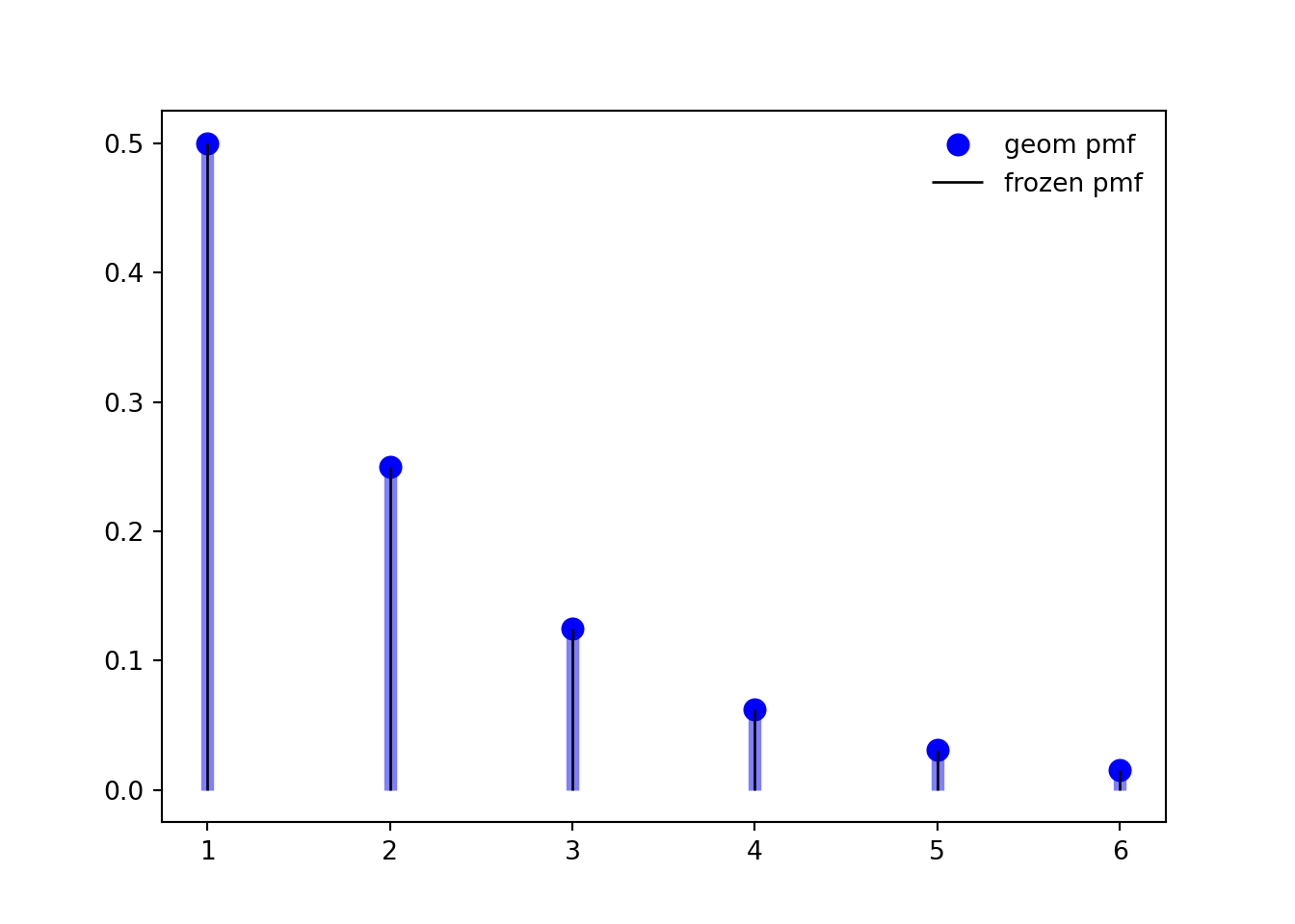
p = 0.5
mean, var, skew, kurt = geom.stats(p,moments='mvsk')
print(f'{mean=:1.2f}, {var=:1.2f}, {skew=:1.2f}, {kurt=:1.2f}')

mean=2.00, var=2.00, skew=2.12, kurt=6.50

x = np.arange(geom.ppf(0.01, p),
              geom.ppf(0.99, p))
ax.plot(x, geom.pmf(x, p), 'bo', ms=8, label='geom pmf')
ax.vlines(x, 0, geom.pmf(x, p), colors='b', lw=5, alpha=0.5)

rv = geom(p)
ax.vlines(x, 0, rv.pmf(x), colors='k', linestyles='-', lw=1,
        label='frozen pmf')
ax.legend(loc='best', frameon=False)
plt.show()

r = geom.rvs(p,size=10)
r

array([1, 2, 1, 4, 1, 1, 5, 1, 1, 1])

B.7 Negative Binomial Distribution

B.7.1 Story

Note

In a sequence of independent Bernoulli trials with success probability p, if X is the number of failures before the r^th success, then X is said to have the Negative Binomial distribution with parameters r and p, denoted X \sim NBin(r, p).

Both the Binomial and the Negative Binomial distributions are based on independent Bernoulli trials; they differ in the stopping rule and in what they are counting.

The Binomial counts the number of successes in a fixed number of trials; the Negative Binomial counts the number of failures until a fixed number of successes.

In light of these similarities, it comes as no surprise that the derivation of the Negative Binomial PMF bears a resemblance to the corresponding derivation for the Binomial.

B.7.2 Parameters

• r the number of successes.
• p the probability of the Bernoulli trial.

B.7.3 Conditions

Tip

• Count of discrete events
• Non-independent events; it is sometimes said that the events can exhibit contagion, meaning that if one event occurs, it is more likely that another will also occur
• Can model a data-generating process where the variance exceeds the mean
• Fixed amount of time or space in which the events can occur

B.7.4 Examples

• Stamp collection - Suppose there are n types of stamps, which you are collecting one by one, with the goal of getting a complete set. When collecting stamps, the stamp types are random. Assume that each time you collect a stamp, it is equally likely to be any of the n types. What is the expected number of toys needed until you have a complete set?
• everything the Poisson can do and more,
• to model the number of measles cases that occur on an island,
• the number of banks that collapse in a financial crisis.
• the length of a hospital stay
• the probability you will have to visit Y houses if you must sell r cookies before returning home

B.7.5 Moments

\mathrm{E}(X) = \lambda

var(X) = \lambda + \frac{\lambda^2}{\kappa}

B.7.6 Probability mass function (PMF)

f(x \mid \lambda,\kappa) = \frac{\Gamma(x+\kappa)}{x!\Gamma(\kappa+1)}\left(\frac{\lambda}{\lambda+\kappa}\right)^x \left(\frac{\kappa}{\lambda+\kappa}\right)^\kappa

B.7.7 Cumulative distribution function (CDF)

F(x \mid \lambda,\kappa) = \begin{cases} I_{\frac{\kappa}{\kappa+\lambda}}(\kappa,1+\lfloor x \rfloor), & x \ge q 0 \\ 0, & \text{Otherwise} \end{cases}

\text{where } I_w(u,v) \text{ is the regularised incomplete beta function: } I_w(u,v) = \frac{B(w; u, v)}{B(u,v)}

\text{where } B(w; u,v)=\int_{0}^{w}t^{u-1}(1-t)^{v-1}\mathrm{d}t \text{ is the incomplete beta function and }\\ B(u,v)=\int_{0}^{1}t^{u-1}(1-t)^{v-1}\mathrm{d}t \text{ is the complete beta function}

B.8 Multinomial Distribution

The Multinomial distribution is a generalization of the Binomial. Whereas the Binomial distribution counts the successes in a fixed number of trials that can only be categorized as success or failure, the Multinomial distribution keeps track of trials whose outcomes can fall into multiple categories, such as excellent, adequate, poor; or red, yellow, green, blue.

B.8.1 Story

Multinomial distribution. Each of N objects is independently placed into one of k categories. An object is placed into category j with probability p_j ,P where the p_j are non-negative and \sum^k_{j=1} p_j = 1. Let X_1 be the number of objects in category 1, X_2 the number of objects in category 2, etc., so that X_1 + \dots + X_k = n. Then X = (X_1 , \dots , X_k ) is said to have the Multinomial distribution with parameters n and p = (p_1 , \dots , p_k ). We write this as X \sim Mult_k(n, p).

We call X a random vector because it is a vector of random variables. The joint PMF of X can be derived from the story.

B.8.2 Examples

• Blood type counts across n individuals
• Numbers of people voting for each party in a sample

B.8.3 Moments

\mathrm{E}(X_i) = n p_i \text{, }\forall i

var(X_i) = n p_i (1-p_i) \text{, }\forall i

cov(X_i,X_j) = -n p_i p_j \text{, }\forall i\neq j

B.8.4 Probability Mass Function (PMF)

f(x_1,x_2,\dots,x_d \mid n,p_1,p_2,\dots,p_d) = \frac{n!}{x_1 ! x_2 ! \dots x_d !} p_1^{x_1} p_2^{x_2}\dots p_d^{x_d}

B.9 Beta Binomial

B.9.1 Story 1 - Polya Urn Model

The beta-binomial distribution with parameters \alpha success rate and \beta failure and n the number of trials can be motivated by an Pólya urn model.

Imagine an urn containing \alpha red balls and \beta black balls, where random draws are made. If a red ball is observed, then two red balls are returned to the urn. Likewise, if a black ball is drawn, then two black balls are returned to the urn. If this is repeated n times, then the probability of observing x red balls follows a beta-binomial distribution with parameters n, \alpha and \beta.

If the random draws are with simple replacement (no balls over and above the observed ball are added to the urn), then the distribution follows a binomial distribution and if the random draws are made without replacement, the distribution follows a hypergeometric distribution.

B.9.2 Story 2 compound distribution

The Beta distribution is a conjugate distribution of the binomial distribution. This fact leads to an analytically tractable compound distribution constructed in a hierarchical fashion where one can think of the p parameter in the binomial distribution as being randomly drawn from a beta distribution.

Suppose we were interested in predicting the number of heads, x in n future trials. This is given by

{\displaystyle { \begin{aligned} f(x\mid n,\alpha ,\beta )&=\int _{0}^{1}\mathrm {Bin} (x \mid n,p)\mathrm {Beta} (p\mid \alpha ,\beta )\,dp\\ [6pt]&={n \choose x}{\frac {1}{\mathrm {B} (\alpha ,\beta )}}\int _{0}^{1}p^{x+\alpha -1}(1-p)^{n-x+\beta -1}\,dp \\ [6pt]&={n \choose x}{\frac {\mathrm {B} (x+\alpha ,n-x+\beta )}{\mathrm {B} (\alpha ,\beta )}}. \end{aligned}}}

{\displaystyle f(x\mid n,\alpha ,\beta )={\frac {\Gamma (n+1)}{\Gamma (x+1)\Gamma (n-x+1)}}{\frac {\Gamma (x+\alpha )\Gamma (n-x+\beta )}{\Gamma (n+\alpha +\beta )}}{\frac {\Gamma (\alpha +\beta )}{\Gamma (\alpha )\Gamma (\beta )}}.}

B.9.3 Moments

\mathrm{E}(X) = \frac{n\alpha}{\alpha+\beta} var(X) = \frac{n\alpha\beta(\alpha+\beta+n)}{(\alpha+\beta)^2(\alpha+\beta+1)}

B.9.4 Probability mass function (PMF)

f(x \mid n,\alpha,\beta) = \binom{n}{x}\frac{B(x+\alpha,n-x+\beta)}{B(\alpha,\beta)}

\text{where } B(u,v)=\int_{0}^{1}t^{u-1}(1-t)^{v-1}\mathrm{d}t \text{ is the (complete) beta function }

B.9.5 Cumulative distribution function (CDF)

F(x\mid n,\alpha,\beta) = \begin{cases} 0, & x<0 \\ \binom{n}{x}\frac{B(x+\alpha,n-x+\beta)}{B(\alpha,\beta)} {}_{3}F_2(1,-x,n-x+\beta;n-x-1,1-x-\alpha;1), & 0\leq x \leq n \\ 1, & x>n \end{cases}

\text{where } {}_{3}F_2(a,b,x) \text{ is the generalised hypergeometric function}

B.9.6 Relations

• The Pascal distribution (after Blaise Pascal) is special cases of the negative binomial distribution. Used with an integer-valued stopping-time parameter r
• The Pólya distribution (for George Pólya) is special cases of the negative binomial distribution. Used with a real-valued-valued stopping-time parameter r

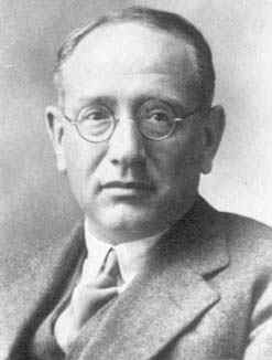
A photo of Hungarian Mathematician George Pólya

TipBiographical note on George Pólya

The cookbook gives a detailed description of ingredients and procedures but no proofs for its prescriptions or reasons for its recipes; the proof of the pudding is in the eating … Mathematics cannot be tested in exactly the same manner as a pudding; if all sorts of reasoning are debarred, a course of calculus may easily become an incoherent inventory of indigestible information. (Polya 1945)

Pólya was arguably the most influential mathematician of the 20th century. His basic research contributions span complex analysis, mathematical physics, probability theory, geometry, and combinatorics. He was a teacher par excellence who maintained a strong interest in pedagogical matters throughout his long career.

He was awarded a doctorate in mathematics having studied, essentially without supervision, a problem in the theory of geometric probability. Later Pólya looked at the Fourier transform of a probability measure, showing in 1923 that it was a characteristic function. He wrote on the normal distribution and coined the term “central limit theorem” in 1920 which is now standard usage.

In 1921 he proved his famous theorem on random walks on an integer lattice. He considered a d-dimensional array of lattice points where a point moves to any of its neighbors with equal probability. He asked whether given an arbitrary point A in the lattice, a point executing a random walk starting from the origin would reach A with probability 1. Pólya’s surprising answer was that it would for d=1 and for d=2, but it would not for d\ge 3. In later work he looked at two points executing independent random walks and also at random walks satisfying the condition that the moving point never passed through the same lattice point twice.

One of Pólya’s notable achievements was his collaboration with the economist Abraham Wald during World War II. They developed statistical techniques to solve military problems, including estimating enemy troop movements and predicting the effectiveness of bombing missions. These contributions played a vital role in aiding the Allies during the war.

His book “How to Solve It,” published in 1945, presented problem-solving heuristics applicable to various mathematical domains, including probability and statistics. This influential work emphasized the importance of understanding the problem, devising a plan, executing the plan, and reflecting on the results. Pólya’s problem-solving strategies continue to be widely taught and practiced.

For a more extensive biography visit the following link

Bernoulli, J. 1713. Ars Conjectandi [the Art of Conjecturing]. Impensis Thurnisiorum.

Polya, G. 1945. How to Solve It. Princeton University Press. https://doi.org/10.1515/9781400828678.