---
date: 2024-11-07
title: "Bayesian Inference in the NDLM: Part 1 M3L7"
subtitle: Time Series Analysis
description: "Normal Dynamic Linear Models (NDLMs) are a class of models used for time series analysis that allow for flexible modeling of temporal dependencies."
categories:
- Bayesian Statistics
- Time Series
keywords:
- Time Series
- Filtering
- Kalman filtering
- Smoothing
- NDLM
- Normal Dynamic Linear Models
- Polynomial Trend Models
- Regression Models
- Superposition Principle
- R code
fig-caption: Notes about ... Bayesian Statistics
title-block-banner: images/banner_deep.jpg
---
:::: {.content-hidden when-format="pdf"}
::: {#vid-sean-law .column-margin}
{{< video https://www.youtube.com/watch?v=0O6dlq6a4rA&ab_channel=SciPy >}}
Sean Law - STUMPY: Modern Time Series Analysis with Matrix Profiles
:::
::::
We will now delve into Bayesian inference for the case where we have an NDLM with both observational variance and system variance known. We will talk about filtering equations, smoothing equations and also forecasting in this setting using Bayesian approach.
::: {.callout-note collapse='false'}
### Reality check {.unnumbered}
1. This lesson is one of several dedicated to Bayesian inference on the NDLM. Professor Prado doesn't outline this study of apparently eclectic collection of NDLM or explain the NDLM framework upfront. It doesn't mean there isn't a method to the madness, however it is up to the student to sort things out.
2. I can say that based on the three prior courses we would follow a similar methodology:
(a) Pick an **[inductive bias](https://en.wikipedia.org/wiki/Inductive_bias** and use it write down some models,
(b) Set a prior
(c) Use Bayes + the data to infer the form of the posterior
(d) Use an algorithm, possibly a Gibbs sampler to approximate the posterior
(e) Recover the parameters by marginalizing the posterior.
(f) ~~Validate convergence of the Algorithm.~~
(g) Validate via prior predictive and posterior predictive checks
(h) Optimize hyperparameters using AIC or BIC
(i) Select the best model via DIC.
Working with AR($p$) loosely followed this process so I expected NDLM would be the same. In the NDLM framework the algorithm is the Kalman Filter. Kalman Filter had originally a Bayesian formulation. The Kalman filter lets us do filtering and smoothing to infer the system parameters we call $\theta_t$. The Kalman filter uses a set of recursive equations to update the state and returns these with an uncertainty estimate! The NDLM framework is mostly a scaffolding to handle the requirements of the Kalman filter (~~discretization of continuous time equations~~, assembling the different part into a single system evolution matrix, converting them into the representation a KF needs, and assembling the different sources of uncertainty i.e. $v$ and $w$ into just one of each per overall model, linearity, ~~controllability~~, setting the boundary conditions from the priors
But I did not know all this. Initially I expected that once we choose a (normal) prior $\mathcal{N}(M_0,\mathbf{C}_0)$ we would infer $\{F,G,V,W\}$ from the data. I supposed that no one has been able to write a prior for $F$ and $G$ and even Kalman in his paper [@kalman1960new] does not describe how to work out the linear system $G$.
While it is never stated explicitly our choice of $F$ and $G$ are very much modeling decisions. $F$ maps the output of $\theta\; G$ and so must be compatible in two sense
1. $F$ must have the same number of rows as $\theta$ has columns
2. $F$ must have the same number of non-zero rows as the output $y_t$
$G$ is the hidden state's evolution matrix. In the NDLM, we don't know very much about the data generating process. Unlike the usual setting for Kalman Filter we don't have access to a dynamical system. All we have is a time series and as modelers we need to construct a surrogate state space model based on very vague prior assumption likely based on some exploration of the time series. (Another problem which could be mitigated via model selection but can also introduce a new issue of too many comparisons if we can choose from too many models)
But this is not the case. In fact we don't seem to be particularly Bayesian when going about constructing the NDLM model.
Similar to constructing a neural network we pick an architecture $\sum \{\mathbf{F}_{i,t},\mathbf{G}_{i,t},\cdot,\cdot\}$
with a hyperparameter like a polynomial degree $q$, an AR($p$) or the number of fourier components $r$ and we give it to the Kalman Filter, which returns an estimate for the $\boldsymbol{\theta}_t$ for us. But that still leaves $\nu_t$ and $\omega_t$.
Now as far as Kalman Filters go $\nu_t$ and $\omega_t$ are errors inherent in the system that cannot be eliminated. One consequence is that our estimates of $theta$ will never converge to the actual state, though they can reach optimality. So as far as the KF is concerned $\nu_t$ and $\omega_t$ are
(i.e. filtering smoothing, of the parameters $\theta_t$ given the data and forecasting $y_t$ based on that)
I was initially disappointed that we assume that we know everything I want to infer. This is an open question for the proverbial [Feynman Notebook](./C4-L06.qmd). In reality that is just another problem.
But that is not the process with time series analysis.
However, at some point I saw a talk about [STUMPY](https://stumpy.readthedocs.io/en/latest/Tutorial_STUMPY_Basics.html) which does many cool time series stuff in python. And the speaker Sean Law talks about all the different Data Science & DSP Mojos `#magicspells` one can use, the nascent issues when comparing lots of times series or even just time series with lots of data. He makes another point that there is `#NoFreeLunch` - each Mojo comes with with its own assumptions and limitations before making the case for using [Matrix Profiles](https://stumpy.readthedocs.io/en/latest/Tutorial_STUMPY_Basics.html).
Prado lays the ground for working with a time series with around 300 data points - i.e. something we can still plot and view on the screen then inspect it. This might unlock for us, the NDLM framework which while flexible requires us to have a detailed form of the the model and its priors. This is easy enough if we deal with a synthetic data set, less so if we have need to analyze an novel time series for which we lack much intuition. Here we will need todo a preliminary exploratory data analysis before we can step in and construct our NDLM.
I suppose they expect that you will use some other non-bayesian tools to do this as we haven't really covered this in her course.
Splitting a TS into trend periods and a stationary residual isn't too tricky in R. Getting the inverse periods is then possible. Doing regression on the residuals is also possible. So if we have done all that we should be able to write down an NDLM based on all that we learned. And this will allow us to do filtering, smoothing and forecasting with error estimates.
p.s. this is a long rant once it's done I think it can be moved to the course intro as an overview of the NDLM part.
:::
## Filtering :movie_camera:
{#fig-derivation-for-the-prior-and-forecast-at-time-t .column-margin group="slides" width="53mm"}
{#fig-derivation-of-the-posterior-at-time-t .column-margin group="slides" width="53mm"}
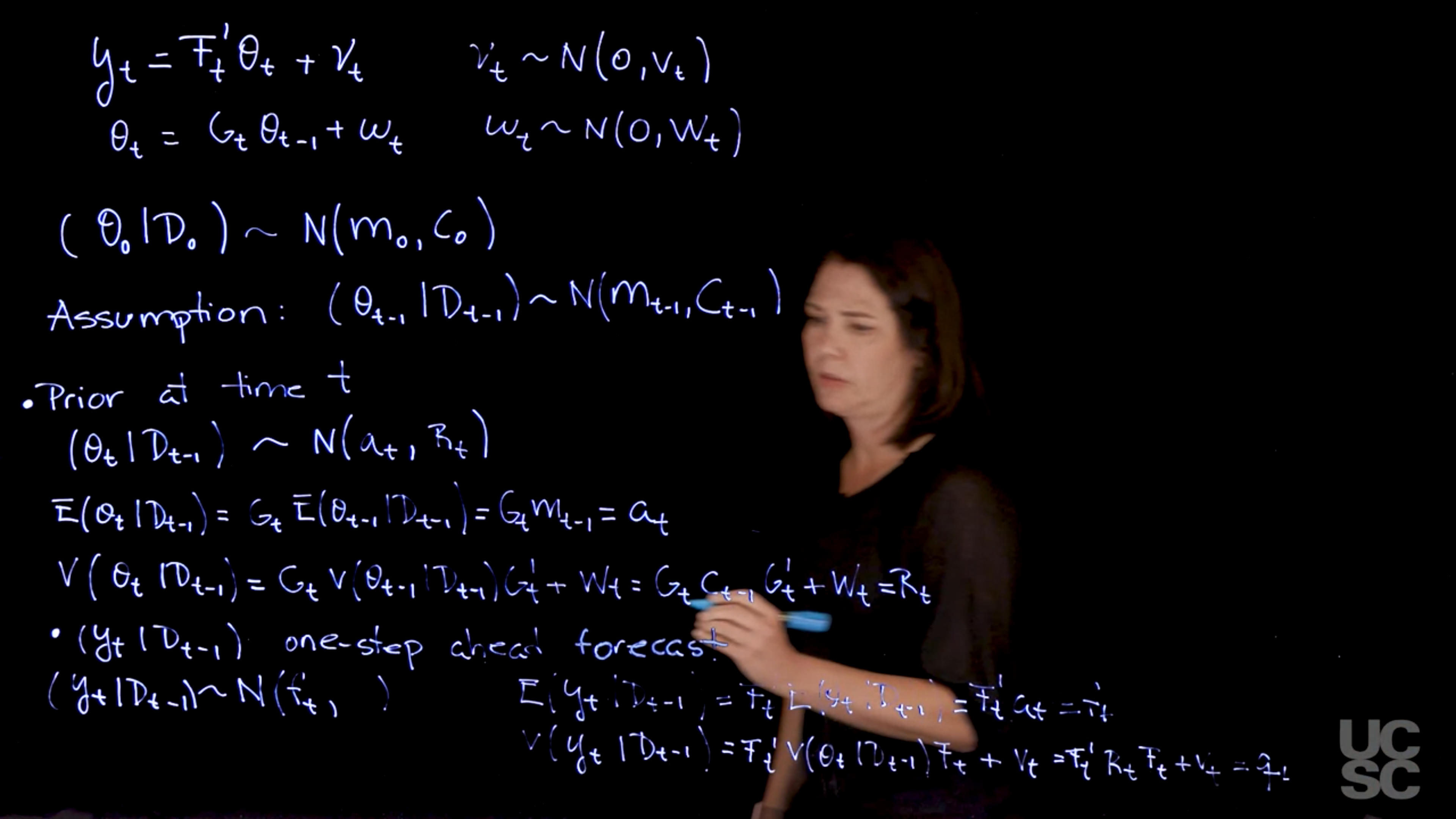
Recall we are working in a Bayesian setting where a NDLM model with a normal prior would like this:
$$
\begin{aligned}
y_t &= F_t' \theta_t + \nu_t & \nu_t &\sim \mathcal{N}(0, v_t) & \text{(observation)} \\
\theta_t &= G_t \theta_{t-1} + \omega_t & \omega_t &\sim \mathcal{N}(0, W_t) & \text{(evolution)} \\
& &(\theta_0 \mid \mathcal{D}_0) & \sim \mathcal{N}(m_0, \mathbf{C}_0) & \text{(prior)}
\end{aligned}
$$ {#eq-generic-NDLM}
- We are assuming:
- $\theta_0 \sim \mathcal{N}(m_0, \mathbf{C}_0)$ variance covariance **matrix**.
- In the prior $\mathcal{D}_0$ denotes the *information set* that we have before collecting any data and
Since we are doing filtering which is a retrospective analysis, of past states we assume that we know $\mathbf{F}_t, \mathbf{G}_t, m_0, \mathbf{C}_0, \nu_t, \omega_t \quad \forall t$.
However, there is often great interest in looking back in time in order to get a clearer picture of what happened.
We are interested in performing Bayesian inference in this setting and we talked about different kinds of distributions.
- One is the **filtering distribution** that allows us to update the distribution of $\theta_t$ as we receive observations and information over time.
- The other one is **smoothing equations** that allows us to just revisit the past once we have observed a chunk of data.
In a Bayesian setting, you have to set *a prior distribution*. [We will work with the prior distribution that is conjugate.]{.mark}
In this case we have to begin with a distribution at time zero for $\theta_0$. So before we have seen any data at all, I have this prior distribution.
We also assume a prior distribution of the form:
$$
(\theta_{t} \mid \mathcal{D}_{t-1}) \sim \mathcal{N}(m_{t-1}, C_{t-1}).
$$ {#eq-filtering-assumption-1}
We assume that this the filtering distribution follows this normal distribution based on
1. the prior in [@eq-generic-NDLM] being conjugate of the normal and
2. the linearity of the model in [@eq-generic-NDLM].
These result in updates to the model parameters and uncertainty, at each time step, preserving the normal structure from the prior.
Then, we can obtain the following distributions:
1. Prior at Time $t$
$$
(\theta_t \mid \mathcal{D}_{t-1}) \sim \mathcal{N}(a_t, R_t) \qquad \text{(prior at time t)} \qquad
$$ {#eq-prior-at-time-t}
with
$$ \begin{aligned}
a_t \doteq& \mathbb{E}[\theta_t \mid \mathcal{D}_{t-1}] =& G_t \mathbb{E}[G_t \theta_{t-1} \mid \mathcal{D}_{t-1} ] =& G_t m_{t-1} \\
R_t \doteq& \mathbb{V}ar[\theta_t \mid \mathcal{D}_{t-1}] =& G_t \mathbb{V}ar[\theta_t \mid \mathcal{D}_{t-1}] =& G_t C_{t-1} G_t' + W_t.
\end{aligned}
$$ {#eq-derivation-for-a-t-and-R-t}
Where we simply took the first and second moments of the system equation from [@eq-generic-NDLM] conditioned on our information set $\mathcal{D}_{t-1}$
2. One-Step Forecast
$$
(y_t \mid \mathcal{D}_{t-1}) \sim \mathcal{N}(f_t, q_t) \quad \text{(one step forecast fn)} \qquad
$$ {#eq-one-step-forecast-fn}
with:
$$
\begin{aligned}
f_t &\doteq \mathbb{E}[ y_t \mid \mathcal{D}_{t-1} ] \\
&= F_t' \; \mathbb{E}[ y_t \mid \mathcal{D}_{t-1} ] \\
&= F_t' \; a_t \\
\end{aligned}
$$ {#eq-derivation-for-f-t}
$$
\begin{aligned}
q_t & \doteq \mathbb{V}ar[y_t \mid \mathcal{D}_{t-1}] \\
&= F_t' \; \mathbb{V}ar[y_t \mid \mathcal{D}_{t-1}] \\
&= F_t' R_t F_t + v_t
\end{aligned}
$$ {#eq-derivation-for-q-t}
Where we took the first moments on the observation equation conditioned on the information set $\mathcal{D}_t$ and substituted @eq-one-step-forecast-fn
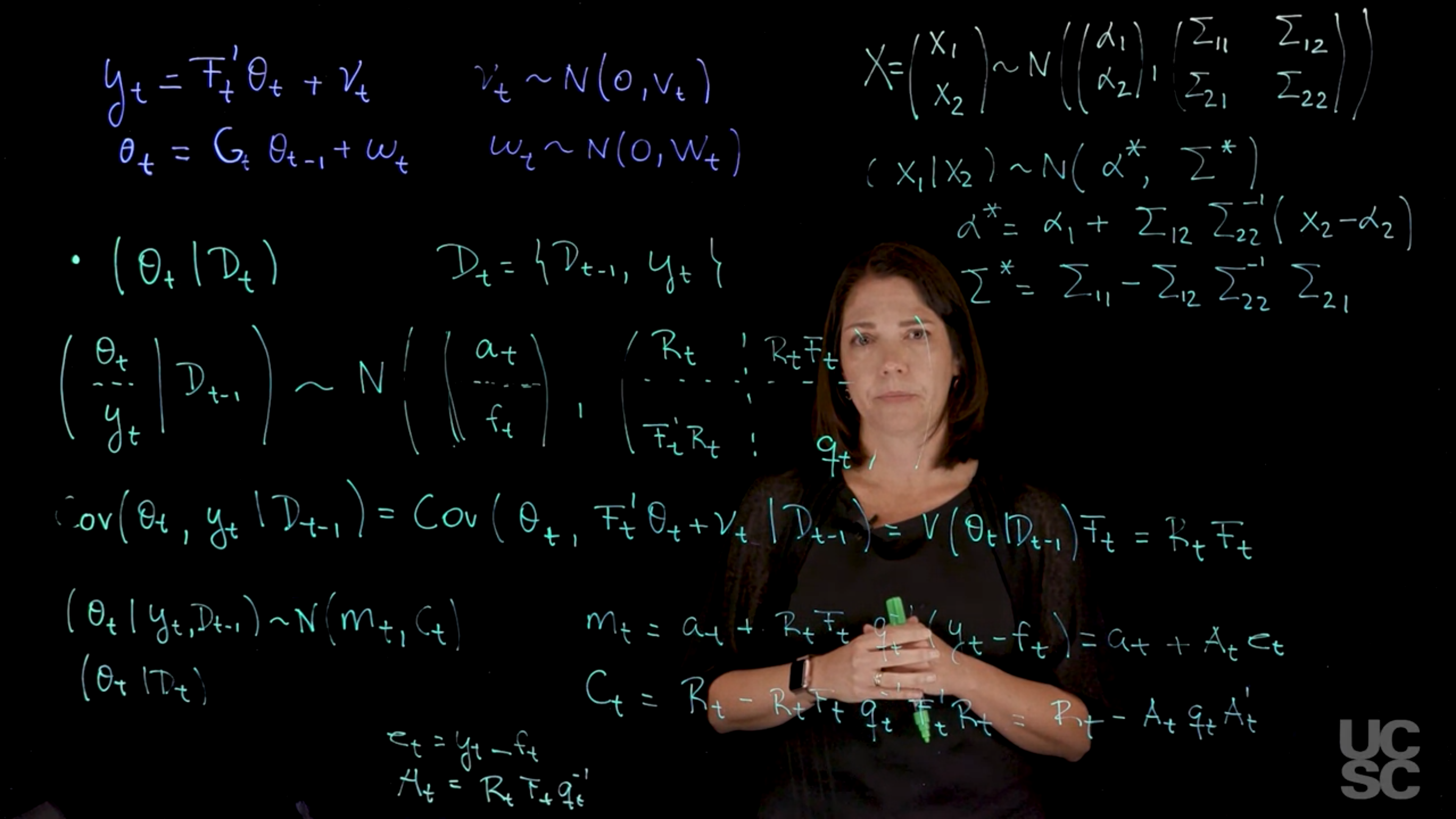
3. Posterior at Time $t$
$$
(\theta_t \mid \mathcal{D}_t) \sim \mathcal{N}(m_t, C_t)
$$
with
$$\begin{aligned}
m_t &= a_t + R_t F_t q_t^{-1} (y_t - f_t), \\
C_t &= R_t - R_t F_t q_t^{-1} F_t' R_t.
\end{aligned}
$$ {#eq-posterior-at-time-t}
These can be derived via Normal theory or via the Multivariate Bayes' theorem. The background for both seems to be provided in [@west2013bayesian §17.2.3 p.639]
Now, denoting $e_t = (y_t - f_t)$ and $A_t = R_t F_t q_t^{-1}$, we can rewrite the equations above as:
It follows that
$$
\begin{pmatrix}Y \\ \theta\end{pmatrix} \sim \mathcal{N}
\left(
\begin{pmatrix}F'a \\ a \end{pmatrix},
\begin{pmatrix} F'RF + V & F'R \\ RF & R \end{pmatrix}
\right)
$$
Therefore, identifying $Y$ with $X_1$ and $\theta$ with $X_2$ in the partition of $X$ in 17.2.2, we have
RF R
)]
Therefore, identifying Y with X1 and $\theta$ with X2 in the partition of X in 17.2.2, we have
$$
Y \sim \mathcal{N}[F'a, F'RF + V]
$$
$$
(\theta \mid Y) \sim \mathcal{N}[m, C],
$$
where
$$
m = a + RF[F′RF + V]−1[Y − F′a]
$$
and
$$
C = R − RF[F′RF + V]−1F′R.
$$
$$
\begin{aligned}
\theta \mid \mathcal{D}_t &\sim \mathcal{N}(m_t,C_t)\\
m_t &\doteq a_t + A_t e_t, \\
C_t &\doteq R_t - A_t q_t A_t'
\end{aligned}
$$ {#eq-posterior-distribution}
@eq-derivation-for-a-t-and-R-t , @eq-derivation-for-f-t-and-q-t and @eq-posterior-distribution are often referred to as the [Kalman filtering](https://en.wikipedia.org/wiki/Kalman_filter) equations.
::: {.callout-note collapse="true"}
## Video Transcript
{{< include transcripts/_C4-L03-T05.qmd >}}
:::
## Summary of filtering distributions :spiral_notepad:
### Bayesian Inference in NDLM: Known Variances
Consider an NDLM given by:
$$
\begin{aligned}
y_t &= F_t' \theta_t + \nu_t, \quad \nu_t \sim \mathcal{N}(0, v_t), \\
\theta_t &= G_t \theta_{t-1} + \omega_t, \quad \omega_t \sim \mathcal{N}(0, W_t),
\end{aligned}
$$ {#eq-generic-NDLM}
with $F_t$, $G_t$, $v_t$, and $W_t$ known. We also assume a prior distribution of the form $(\theta_0 \mid \mathcal{D}_0) \sim \mathcal{N}(m_0, C_0)$, with $m_0$, $C_0$ known.
#### Filtering
We are interested in finding $\mathbb{P}r(\theta_t \mid \mathcal{D}_t)$ for all $t$. Assume that the posterior at $t-1$ is such that:
$$
(\theta_{t-1} \mid \mathcal{D}_{t-1}) \sim \mathcal{N}(m_{t-1}, C_{t-1}).
$$ {#eq-filtering}
Then, we can obtain the following:
1. Prior at Time $t$
$$
(\theta_t \mid \mathcal{D}_{t-1}) \sim \mathcal{N}(a_t, R_t),
$$
with
$$
a_t = G_t m_{t-1} \qquad R_t = G_t C_{t-1} G_t' + W_t.
$$
2. One-Step Forecast
$$
(y_t \mid D_{t-1}) \sim \mathcal{N}(f_t, q_t),
$$
with
$$
f_t = F_t' a_t, \quad q_t = F_t' R_t F_t + v_t.
$$
3. Posterior at Time $t: (\theta_t \mid \mathcal{D}_t) \sim \mathcal{N}(m_t, C_t)$ with
$$\begin{aligned}
m_t &= a_t + R_t F_t q_t^{-1} (y_t - f_t), \\
C_t &= R_t - R_t F_t q_t^{-1} F_t' R_t.
\end{aligned}
$$
Now, denoting $e_t = (y_t - f_t)$ and $A_t = R_t F_t q_t^{-1}$, we can rewrite the equations above as:
$$\begin{aligned}
m_t &= a_t + A_t e_t, \\
C_t &= R_t - A_t q_t A_t'
\end{aligned}
$$
## code Filtering in the NDLM: Example :spiral_notepad: $\mathcal{R}$
```{r}
#| label: lst-filtering-in-the-NDLM
#################################################
##### Univariate DLM: Known, constant variances
#################################################
set_up_dlm_matrices <- function(FF, GG, VV, WW){
return(list(FF=FF, GG=GG, VV=VV, WW=WW))
}
set_up_initial_states <- function(m0, C0){
return(list(m0=m0, C0=C0))
}
### forward update equations ###
forward_filter <- function(data, matrices, initial_states){
## retrieve dataset
y_t <- data$y_t
T <- length(y_t)
## retrieve a set of quadruples
# FF, GG, VV, WW are scalar
FF <- matrices$FF
GG <- matrices$GG
VV <- matrices$VV
WW <- matrices$WW
## retrieve initial states
m0 <- initial_states$m0
C0 <- initial_states$C0
## create placeholder for results
d <- dim(GG)[1]
at <- matrix(NA, nrow=T, ncol=d)
Rt <- array(NA, dim=c(d, d, T))
ft <- numeric(T)
Qt <- numeric(T)
mt <- matrix(NA, nrow=T, ncol=d)
Ct <- array(NA, dim=c(d, d, T))
et <- numeric(T)
for(i in 1:T){
# moments of priors at t
if(i == 1){
at[i, ] <- GG %*% t(m0)
Rt[, , i] <- GG %*% C0 %*% t(GG) + WW
Rt[, , i] <- 0.5*Rt[, , i]+0.5*t(Rt[, , i])
}else{
at[i, ] <- GG %*% t(mt[i-1, , drop=FALSE])
Rt[, , i] <- GG %*% Ct[, , i-1] %*% t(GG) + WW
Rt[, , i] <- 0.5*Rt[, , i]+0.5*t(Rt[, , i])
}
# moments of one-step forecast:
ft[i] <- t(FF) %*% (at[i, ])
Qt[i] <- t(FF) %*% Rt[, , i] %*% FF + VV
# moments of posterior at t:
At <- Rt[, , i] %*% FF / Qt[i]
et[i] <- y_t[i] - ft[i]
mt[i, ] <- at[i, ] + t(At) * et[i]
Ct[, , i] <- Rt[, , i] - Qt[i] * At %*% t(At)
Ct[, , i] <- 0.5*Ct[, , i]+ 0.5*t(Ct[, , i])
}
cat("Forward filtering is completed!") # indicator of completion
return(list(mt = mt, Ct = Ct, at = at, Rt =
Rt, ft = ft, Qt = Qt))
}
forecast_function <- function(posterior_states, k, matrices){
## retrieve matrices
FF <- matrices$FF
GG <- matrices$GG
WW <- matrices$WW
VV <- matrices$VV
mt <- posterior_states$mt
Ct <- posterior_states$Ct
## set up matrices
T <- dim(mt)[1] # time points
d <- dim(mt)[2] # dimension of state-space parameter vector
## placeholder for results
at <- matrix(NA, nrow = k, ncol = d)
Rt <- array(NA, dim=c(d, d, k))
ft <- numeric(k)
Qt <- numeric(k)
for(i in 1:k){
## moments of state distribution
if(i == 1){
at[i, ] <- GG %*% t(mt[T, , drop=FALSE])
Rt[, , i] <- GG %*% Ct[, , T] %*% t(GG) + WW
Rt[, , i] <- 0.5*Rt[, , i]+0.5*t(Rt[, , i])
}else{
at[i, ] <- GG %*% t(at[i-1, , drop=FALSE])
Rt[, , i] <- GG %*% Rt[, , i-1] %*% t(GG) + WW
Rt[, , i] <- 0.5*Rt[, , i]+0.5*t(Rt[, , i])
}
## moments of forecast distribution
ft[i] <- t(FF) %*% t(at[i, , drop=FALSE])
Qt[i] <- t(FF) %*% Rt[, , i] %*% FF + VV
}
cat("Forecasting is completed!") # indicator of completion
return(list(at=at, Rt=Rt, ft=ft, Qt=Qt))
}
## obtain 95% credible interval
get_credible_interval <- function(mu, sigma2,
quantile = c(0.025, 0.975)){
z_quantile <- qnorm(quantile)
bound <- matrix(0, nrow=length(mu), ncol=2)
bound[, 1] <- mu +
z_quantile[1]*sqrt(as.numeric(sigma2)) # lower bound
bound[, 2] <- mu +
z_quantile[2]*sqrt(as.numeric(sigma2)) # upper bound
return(bound)
}
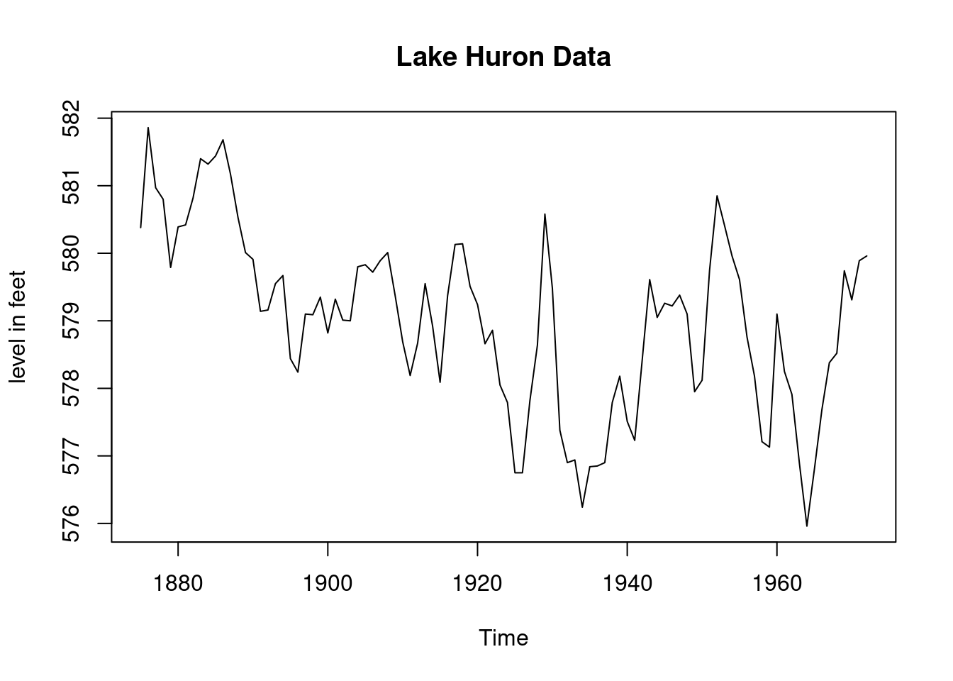
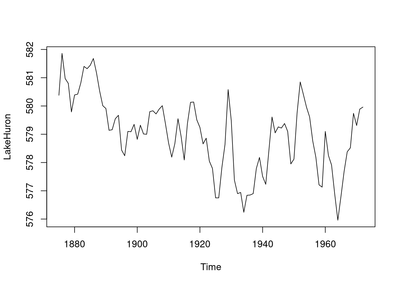
####################### Example: Lake Huron Data ######################
plot(LakeHuron,main="Lake Huron Data",
ylab="level in feet") # Total of 98 observations
k=4
T=length(LakeHuron)-k # We take the first 94 observations
                      # only as our data
ts_data=LakeHuron[1:T]
ts_validation_data <- LakeHuron[(T+1):98]

data <- list(y_t = ts_data)

# First order polynomial model

## set up the DLM matrices
FF <- as.matrix(1)
GG <- as.matrix(1)
VV <- as.matrix(1)
WW <- as.matrix(1)
m0 <- as.matrix(570)
C0 <- as.matrix(1e4)

## wrap up all matrices and initial values
matrices <- set_up_dlm_matrices(FF, GG, VV, WW)
initial_states <- set_up_initial_states(m0, C0)

## filtering
results_filtered <- forward_filter(data, matrices,
                                   initial_states)
names(results_filtered)
ci_filtered <- get_credible_interval(results_filtered$mt,
                                     results_filtered$Ct)

## forecasting
results_forecast <- forecast_function(results_filtered,k,
                                      matrices)
ci_forecast <- get_credible_interval(results_forecast$ft,
results_forecast$Qt)
index=seq(1875, 1972, length.out = length(LakeHuron))
index_filt=index[1:T]
index_forecast=index[(T+1):98]
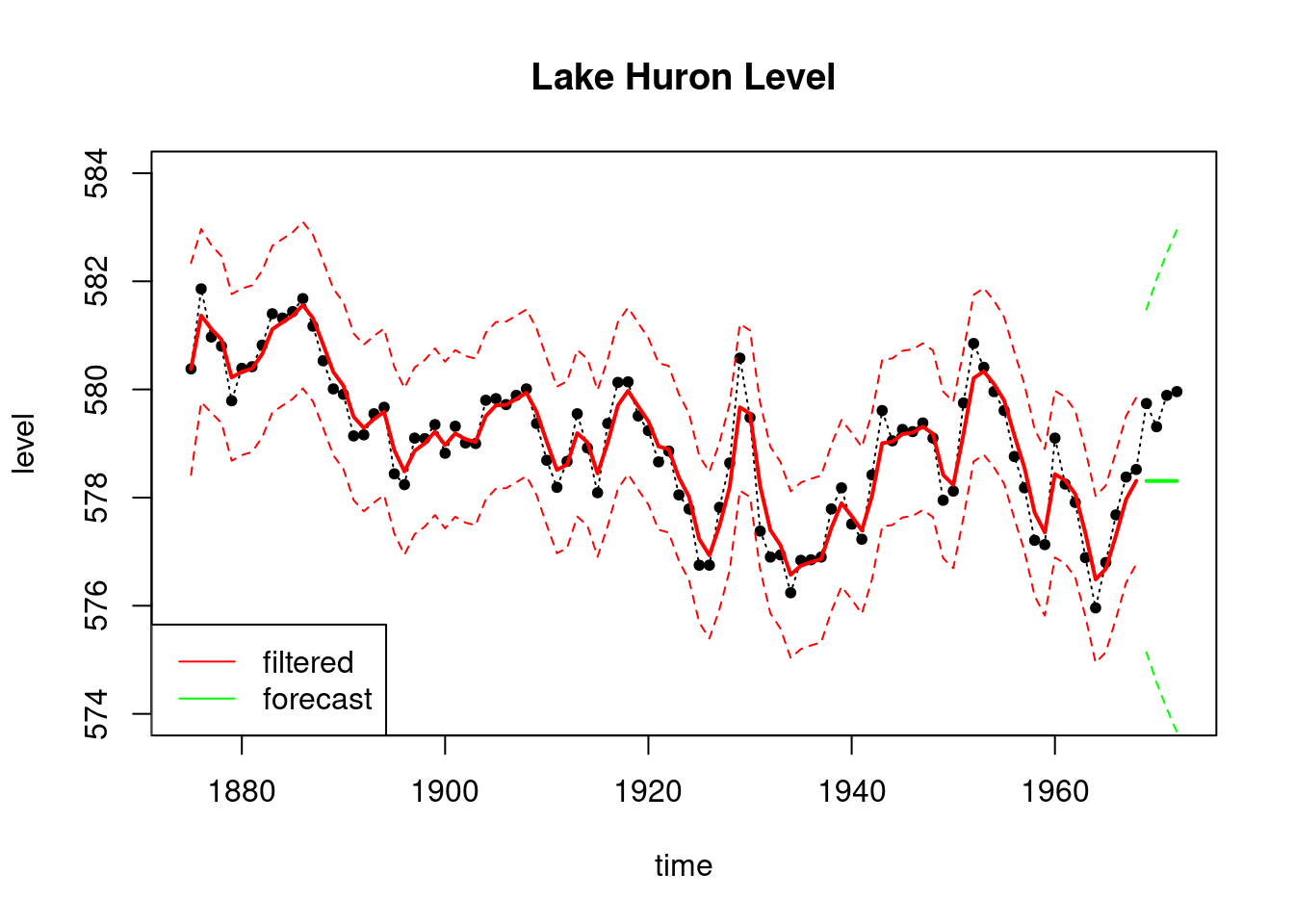
plot(index, LakeHuron, ylab = "level",
main = "Lake Huron Level",type='l',
xlab="time",lty=3,ylim=c(574,584))
points(index,LakeHuron,pch=20)
lines(index_filt, results_filtered$mt, type='l',
col='red',lwd=2)
lines(index_filt, ci_filtered[, 1], type='l',
col='red', lty=2)
lines(index_filt, ci_filtered[, 2], type='l', col='red', lty=2)
lines(index_forecast, results_forecast$ft, type='l',
col='green',lwd=2)
lines(index_forecast, ci_forecast[, 1], type='l',
col='green', lty=2)
lines(index_forecast, ci_forecast[, 2], type='l',
col='green', lty=2)
legend('bottomleft', legend=c("filtered","forecast"),
col = c("red", "green"), lty=c(1, 1))
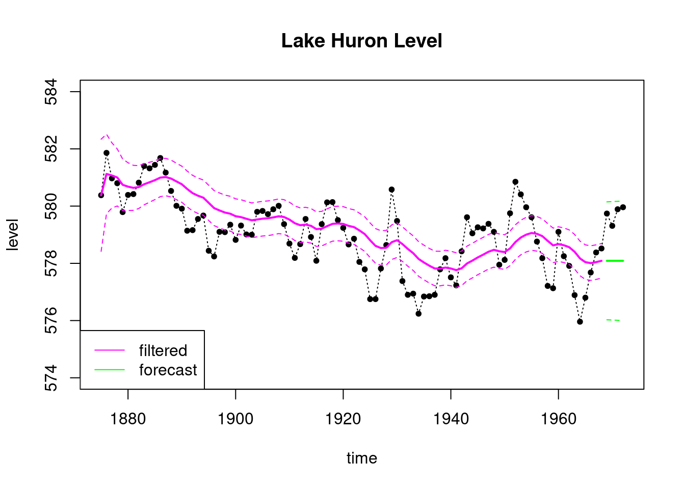
#Now consider a 100 times smaller signal to noise ratio
VV <- as.matrix(1)
WW <- as.matrix(0.01)
matrices_2 <- set_up_dlm_matrices(FF,GG, VV, WW)

## filtering
results_filtered_2 <- forward_filter(data, matrices_2,
                                     initial_states)
ci_filtered_2 <- get_credible_interval(results_filtered_2$mt,
                                       results_filtered_2$Ct)

results_forecast_2 <- forecast_function(results_filtered_2,
                             length(ts_validation_data),
                             matrices_2)
ci_forecast_2 <- get_credible_interval(results_forecast_2$ft,
                                       results_forecast_2$Qt)


plot(index, LakeHuron, ylab = "level",
     main = "Lake Huron Level",type='l',
     xlab="time",lty=3,ylim=c(574,584))
points(index,LakeHuron,pch=20)

lines(index_filt, results_filtered_2$mt, type='l',
      col='magenta',lwd=2)
lines(index_filt, ci_filtered_2[, 1], type='l',
      col='magenta', lty=2)
lines(index_filt, ci_filtered_2[, 2], type='l',
      col='magenta', lty=2)

lines(index_forecast, results_forecast_2$ft, type='l',
      col='green',lwd=2)
lines(index_forecast, ci_forecast_2[, 1], type='l',
      col='green', lty=2)
lines(index_forecast, ci_forecast_2[, 2], type='l',
      col='green', lty=2)

legend('bottomleft', legend=c("filtered","forecast"),
       col = c("magenta", "green"), lty=c(1, 1))
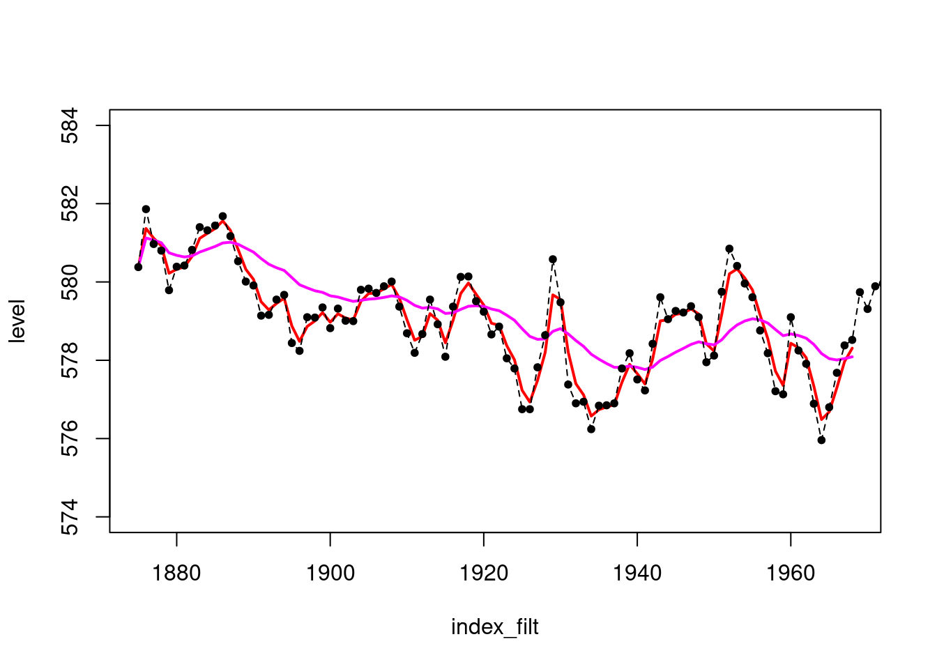
plot(index_filt,results_filtered$mt,type='l',col='red',lwd=2,
     ylim=c(574,584),ylab="level")
lines(index_filt,results_filtered_2$mt,col='magenta',lwd=2)
points(index,LakeHuron,pch=20)
lines(index,LakeHuron,lty=2)
```
## Smoothing and forecasting :movie_camera:
{#fig-smoothing .column-margin group="slides" width="53mm"}
{#fig-forecasting .column-margin group="slides" width="53mm"}
We now discuss the **smoothing equations** for the case of the NDLM, where we are assuming that the variance at the *observation level* $\nu_t$ and the covariance matrix at the *system level* $\mathbf{W}_t$ are both known.
$$ \begin{aligned}
y_t &= \mathbf{F}_t' \mathbf{\theta}_t + \nu_t, &\nu_t &\sim \mathcal{N} (0, v_t), & \text{(observation)} \\
\mathbf{\theta}_t & = \mathbf{G}_t \mathbf{\theta}_{t-1} + \mathbf{\omega}_t, &\mathbf{\omega}_t & \sim \mathcal{N} (0, \mathbf{W}_t), & \text{(evolution)} \\
&\{ \mathbf{F}_t, \mathbf{G}_t, v_t, \mathbf{W}_t \} &(\mathbf{\omega}_0 \mid \mathcal{D}_0) & \sim \mathcal{N}(\mathbf{m}_0, \mathbf{C}_0) & \text{(prior)}
\end{aligned}
$$ {#eq-inference-NDLM}
with $F_t$, $G_t$, $v_t$, $W_t$, $m_0$ and $C_0$ known.
We have discussed the filtering equations, i.e. the process for obtaining the distributions of $\theta_t \mid \mathcal{D}_t$, as we collect observations over time, called filtering.
We do this by updating the distribution of $\theta_t$ given the data we have collected step by step, as we move forward in time - updating the from the prior distribution.
Now we will discuss what happens when we do smoothing, meaning when we revisit the distributions of $\theta_t$, given now that we have received a set of observations.
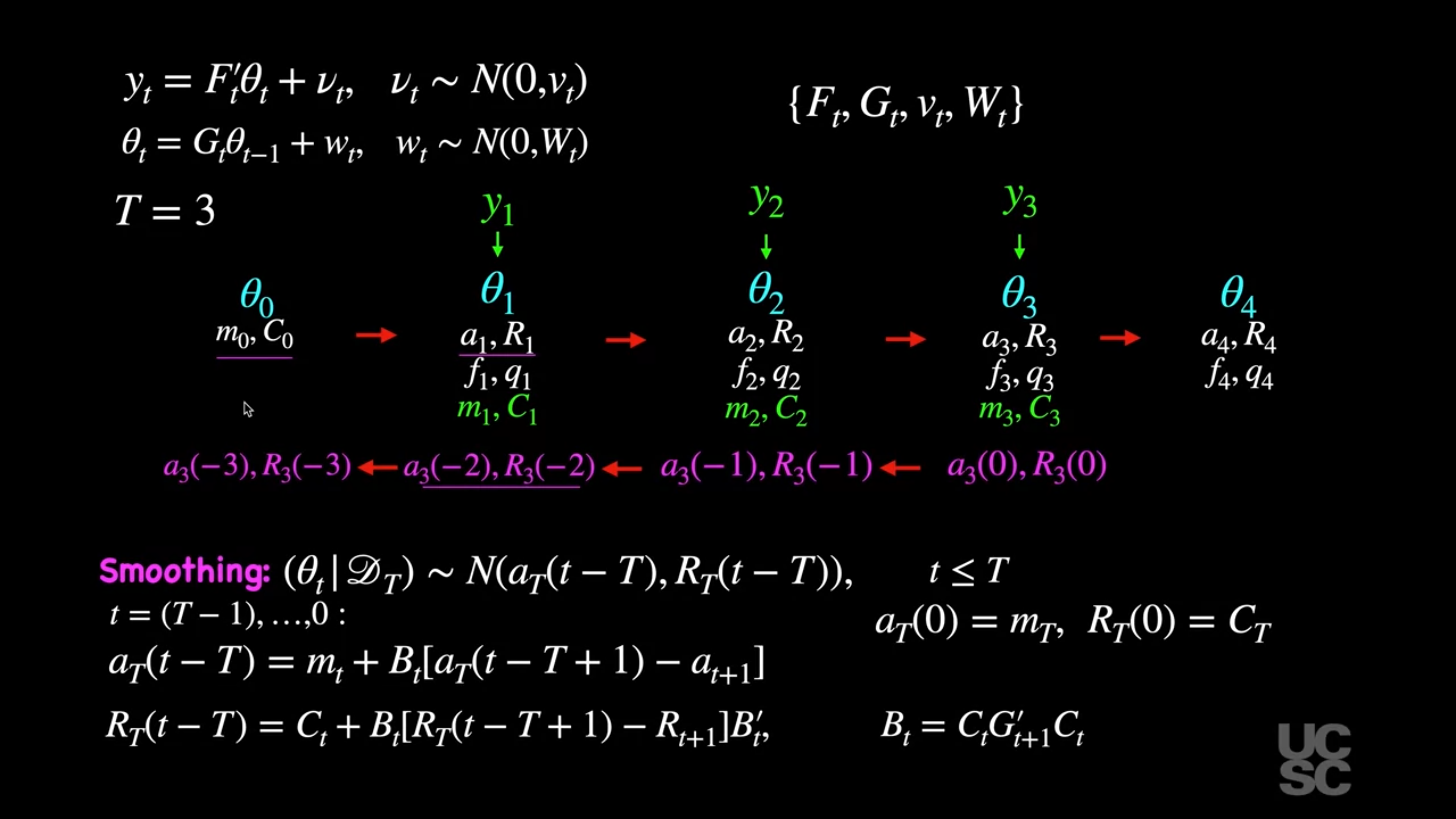
#### Smoothing
For $t < T$, we have that:
$$
(\theta_t \mid D_T) \sim \mathcal{N}(a_T(t - T), R_T(t - T)),
$$
where
$$
a_T(t - T) = m_t - B_t [a_{t+1} - a_T(t - T + 1)],
$$
$$
R_T(t - T) = C_t - B_t [R_{t+1} - R_T(t - T + 1)] B_t',
$$
for $t = (T - 1), (T - 2), \dots, 0$, with $B_t = C_t G_t' R_{t+1}^{-1}$, and $a_T(0) = m_T$, $R_T(0) = C_T$. Here $a_t$, $m_t$, $R_t$, and $C_t$ are obtained using the filtering equations as explained before.
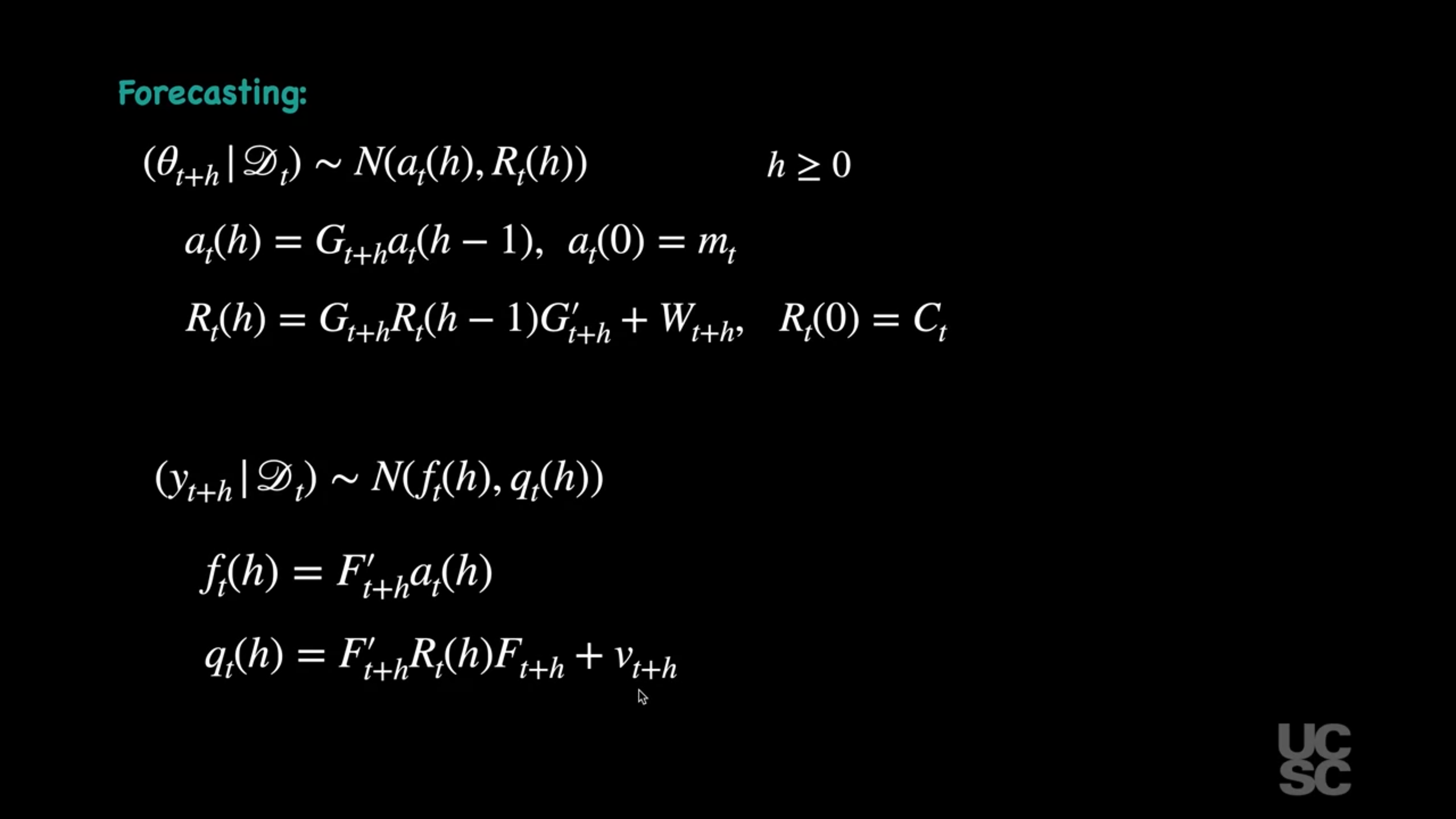
#### Forecasting
For $h \geq 0$, it is possible to show that:
$$
(\theta_{t+h} \mid D_t) \sim \mathcal{N}(a_t(h), R_t(h)),
$$
$$
(y_{t+h} \mid D_t) \sim \mathcal{N}(f_t(h), q_t(h)),
$$
with
$$
a_t(h) = G_{t+h} a_t(h - 1),
$$
$$
R_t(h) = G_{t+h} R_t(h - 1) G_{t+h}' + W_{t+h},
$$
$$
f_t(h) = F_{t+h}' a_t(h),
$$
$$
q_t(h) = F_{t+h}' R_t(h) F_{t+h} + v_{t+h},
$$
and
$$
a_t(0) = m_t, \quad R_t(0) = C_t.
$$
::: {.callout-note collapse="true"}
## Video Transcript
{{< include transcripts/_C4-L03-T06.qmd >}}
:::
## Summary of the smoothing and forecasting distributions :spiral_notepad: {#sec-summary-smoothing-forecasting}
<!-- start -->
### Bayesian Inference in NDLM: Known Variances {#sec-Bayesian-inference-NDLM-known-variances}
Consider the NDLM given by:
$$ \begin{aligned}
y_t &= \mathbf{F}_t' \mathbf{\theta}_t + \nu_t, &\nu_t &\sim \mathcal{N} (0, v_t), \\
\mathbf{\theta}_t &= \mathbf{G}_t \mathbf{\theta}_{t-1} + \mathbf{\omega}_t, &\mathbf{\omega}_t &\sim \mathcal{N} (0, \mathbf{W}_t), \\
&\{\textcolor{green}{\mathbf{F}_t, \mathbf{G}_t, v_t, \mathbf{W}_t} \} &(\mathbf{\omega}_0 \mid \mathcal{D}_0) &\sim \mathcal{N}(\textcolor{green}{\mathbf{m}_0, \mathbf{C}_0})
\end{aligned}
$$ {#eq-inference-NDLM}
with $F_t$, $G_t$, $v_t$, and $W_t$ known.
We also assume a prior distribution of the form
$(\theta_0 \mid D_0) \sim \mathcal{N}(m_0, C_0)$, with $m_0$ and $C_0$ known.
Let's reflect for a moment on the assumption about known quantities (in green):
$F_t$, $G_t$, are modeling choices as are the parameters of the prior $m_0$, and $C_0$.
#### Smoothing
For $t < T$, we have that:
$$
(\theta_t \mid D_T) \sim \mathcal{N}(a_T(t - T), R_T(t - T)),
$$
where
$$
a_T(t - T) = m_t - B_t [a_{t+1} - a_T(t - T + 1)],
$$
$$
R_T(t - T) = C_t - B_t [R_{t+1} - R_T(t - T + 1)] B_t',
$$
for $t = (T - 1), (T - 2), \dots, 0$, with $B_t = C_t G_t' R_{t+1}^{-1}$, and $a_T(0) = m_T$, $R_T(0) = C_T$. Here $a_t$, $m_t$, $R_t$, and $C_t$ are obtained using the filtering equations as explained before.
#### Forecasting
For $h \geq 0$, it is possible to show that:
$$
(\theta_{t+h} \mid D_t) \sim \mathcal{N}(a_t(h), R_t(h)),
$$
$$
(y_{t+h} \mid D_t) \sim \mathcal{N}(f_t(h), q_t(h)),
$$
with
$$
a_t(h) = G_{t+h} a_t(h - 1),
$$
$$
R_t(h) = G_{t+h} R_t(h - 1) G_{t+h}' + W_{t+h},
$$
$$
f_t(h) = F_{t+h}' a_t(h),
$$
$$
q_t(h) = F_{t+h}' R_t(h) F_{t+h} + v_{t+h},
$$
and
$$
a_t(0) = m_t, \quad R_t(0) = C_t.
$$
<!-- end -->
## Smoothing in the NDLM, Example :movie_camera:
This segment covers the code in the following section
## Code: Smoothing in the NDLM, Example :spiral_notepad: $\mathcal{R}$ {#sec-smoothing-in-the-NDLM}
```{r}
#| label: lst-smoothing-in-the-NDLM
#################################################
##### Univariate DLM: Known, constant variances
#################################################
set_up_dlm_matrices <- function(FF, GG, VV, WW){
  return(list(FF=FF, GG=GG, VV=VV, WW=WW))
}

set_up_initial_states <- function(m0, C0){
  return(list(m0=m0, C0=C0))
}

### forward update equations ###
forward_filter <- function(data, matrices, initial_states){
  ## retrieve dataset
  y_t <- data$y_t
  T <- length(y_t)

  ## retrieve a set of quadruples
  # FF, GG, VV, WW are scalar
  FF <- matrices$FF
  GG <- matrices$GG
  VV <- matrices$VV
  WW <- matrices$WW

  ## retrieve initial states
  m0 <- initial_states$m0
  C0 <- initial_states$C0

  ## create placeholder for results
  d <- dim(GG)[1]
  at <- matrix(NA, nrow=T, ncol=d)
  Rt <- array(NA, dim=c(d, d, T))
  ft <- numeric(T)
  Qt <- numeric(T)
  mt <- matrix(NA, nrow=T, ncol=d)
  Ct <- array(NA, dim=c(d, d, T))
  et <- numeric(T)


  for(i in 1:T){
    # moments of priors at t
    if(i == 1){
      at[i, ] <- GG %*% t(m0)
      Rt[, , i] <- GG %*% C0 %*% t(GG) + WW
      Rt[,,i] <- 0.5*Rt[,,i]+0.5*t(Rt[,,i])
    }else{
      at[i, ] <- GG %*% t(mt[i-1, , drop=FALSE])
      Rt[, , i] <- GG %*% Ct[, , i-1] %*% t(GG) + WW
      Rt[,,i] <- 0.5*Rt[,,i]+0.5*t(Rt[,,i])
    }

    # moments of one-step forecast:
    ft[i] <- t(FF) %*% (at[i, ])
    Qt[i] <- t(FF) %*% Rt[, , i] %*% FF + VV

    # moments of posterior at t:
    At <- Rt[, , i] %*% FF / Qt[i]
    et[i] <- y_t[i] - ft[i]
    mt[i, ] <- at[i, ] + t(At) * et[i]
    Ct[, , i] <- Rt[, , i] - Qt[i] * At %*% t(At)
    Ct[,,i] <- 0.5*Ct[,,i] + 0.5*t(Ct[,,i])
  }
  cat("Forward filtering is completed!") # indicator of completion
  return(list(mt = mt, Ct = Ct, at = at, Rt = Rt,
              ft = ft, Qt = Qt))
}


forecast_function <- function(posterior_states, k, matrices){

  ## retrieve matrices
  FF <- matrices$FF
  GG <- matrices$GG
  WW <- matrices$WW
  VV <- matrices$VV
  mt <- posterior_states$mt
  Ct <- posterior_states$Ct

  ## set up matrices
  T <- dim(mt)[1] # time points
  d <- dim(mt)[2] # dimension of state parameter vector

  ## placeholder for results
  at <- matrix(NA, nrow = k, ncol = d)
  Rt <- array(NA, dim=c(d, d, k))
  ft <- numeric(k)
  Qt <- numeric(k)


  for(i in 1:k){
    ## moments of state distribution
    if(i == 1){
      at[i, ] <- GG %*% t(mt[T, , drop=FALSE])
      Rt[, , i] <- GG %*% Ct[, , T] %*% t(GG) + WW
      Rt[,,i] <- 0.5*Rt[,,i]+0.5*t(Rt[,,i])
    }else{
      at[i, ] <- GG %*% t(at[i-1, , drop=FALSE])
      Rt[, , i] <- GG %*% Rt[, , i-1] %*% t(GG) + WW
      Rt[,,i] <- 0.5*Rt[,,i]+0.5*t(Rt[,,i])
    }

    ## moments of forecast distribution
    ft[i] <- t(FF) %*% t(at[i, , drop=FALSE])
    Qt[i] <- t(FF) %*% Rt[, , i] %*% FF + VV
  }
  cat("Forecasting is completed!") # indicator of completion
  return(list(at=at, Rt=Rt, ft=ft, Qt=Qt))
}

## obtain 95% credible interval
get_credible_interval <- function(mu, sigma2,
                          quantile = c(0.025, 0.975)){
  z_quantile <- qnorm(quantile)
  bound <- matrix(0, nrow=length(mu), ncol=2)
  bound[, 1] <- mu + z_quantile[1]*sqrt(as.numeric(sigma2)) # lower bound
  bound[, 2] <- mu + z_quantile[2]*sqrt(as.numeric(sigma2)) # upper bound
  return(bound)
}

### smoothing equations ###
backward_smoothing <- function(data, matrices,
                               posterior_states){
  ## retrieve data
  y_t <- data$y_t
  T <- length(y_t)

  ## retrieve matrices
  FF <- matrices$FF
  GG <- matrices$GG

  ## retrieve matrices
  mt <- posterior_states$mt
  Ct <- posterior_states$Ct
  at <- posterior_states$at
  Rt <- posterior_states$Rt

  ## create placeholder for posterior moments
  mnt <- matrix(NA, nrow = dim(mt)[1], ncol = dim(mt)[2])
  Cnt <- array(NA, dim = dim(Ct))
  fnt <- numeric(T)
  Qnt <- numeric(T)
  for(i in T:1){
    # moments for the distributions of the state vector given D_T
    if(i == T){
      mnt[i, ] <- mt[i, ]
      Cnt[, , i] <- Ct[, , i]
      Cnt[, , i] <- 0.5*Cnt[, , i] + 0.5*t(Cnt[, , i])
    }else{
      inv_Rtp1<-solve(Rt[,,i+1])
      Bt <- Ct[, , i] %*% t(GG) %*% inv_Rtp1
      mnt[i, ] <- mt[i, ] + Bt %*% (mnt[i+1, ] - at[i+1, ])
      Cnt[, , i] <- Ct[, , i] + Bt %*% (Cnt[, , i + 1] - Rt[, , i+1]) %*% t(Bt)
      Cnt[,,i] <- 0.5*Cnt[,,i] + 0.5*t(Cnt[,,i])
    }
    # moments for the smoothed distribution of the mean response of the series
    fnt[i] <- t(FF) %*% t(mnt[i, , drop=FALSE])
    Qnt[i] <- t(FF) %*% t(Cnt[, , i]) %*% FF
  }
  cat("Backward smoothing is completed!")
  return(list(mnt = mnt, Cnt = Cnt, fnt=fnt, Qnt=Qnt))
}
####################### Example: Lake Huron Data ######################
plot(LakeHuron,main="Lake Huron Data",ylab="level in feet")
# 98 observations total
k=4
T=length(LakeHuron)-k # We take the first 94 observations
                     #  as our data
ts_data=LakeHuron[1:T]
ts_validation_data <- LakeHuron[(T+1):98]

data <- list(y_t = ts_data)

## set up matrices
FF <- as.matrix(1)
GG <- as.matrix(1)
VV <- as.matrix(1)
WW <- as.matrix(1)
m0 <- as.matrix(570)
C0 <- as.matrix(1e4)

## wrap up all matrices and initial values
matrices <- set_up_dlm_matrices(FF,GG,VV,WW)
initial_states <- set_up_initial_states(m0, C0)

## filtering
results_filtered <- forward_filter(data, matrices,
                                   initial_states)
ci_filtered<-get_credible_interval(results_filtered$mt,
                                   results_filtered$Ct)
## smoothing
results_smoothed <- backward_smoothing(data, matrices,
                                       results_filtered)
ci_smoothed <- get_credible_interval(results_smoothed$mnt,
results_smoothed$Cnt)
index=seq(1875, 1972, length.out = length(LakeHuron))
index_filt=index[1:T]
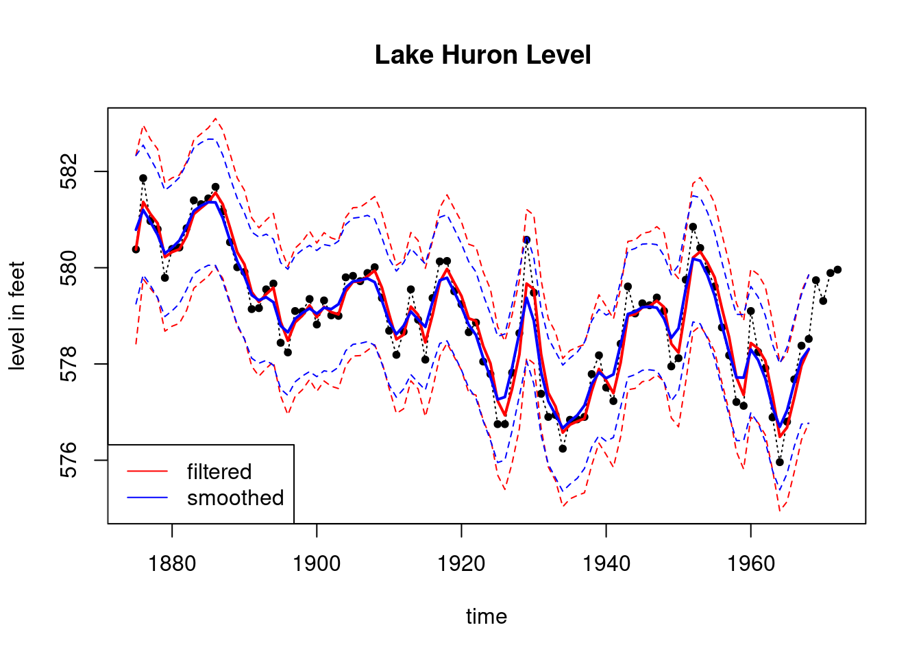
plot(index, LakeHuron, main = "Lake Huron Level ",type='l',
xlab="time",ylab="level in feet",lty=3,ylim=c(575,583))
points(index,LakeHuron,pch=20)
lines(index_filt, results_filtered$mt, type='l',
col='red',lwd=2)
lines(index_filt, ci_filtered[,1], type='l', col='red',lty=2)
lines(index_filt, ci_filtered[,2], type='l', col='red',lty=2)
lines(index_filt, results_smoothed$mnt, type='l',
col='blue',lwd=2)
lines(index_filt, ci_smoothed[,1], type='l', col='blue',lty=2)
lines(index_filt, ci_smoothed[,2], type='l', col='blue',lty=2)
legend('bottomleft', legend=c("filtered","smoothed"),
col = c("red", "blue"), lty=c(1, 1))
```
## Second order polynomial: Filtering and smoothing example :movie_camera: {#sec-second-order-polynomial}
In this video walk through the code provided in the section below the comment
::: {.callout-note collapse="true"}
## Video Transcript
{{< include transcripts/_C4-L03-T07.qmd >}}
:::
## Using the `DLM` package in R :movie_camera:
The `DLM` library in R is a powerful tool for working with dynamic linear models. The package provides a wide range of functions for filtering, smoothing, forecasting, and parameter estimation in DLMs. In this video, we walk through the code provided in @lst-dlm-package.
::: {.callout-note collapse="true"}
## Video Transcript
{{< include transcripts/_C4-L03-T08.qmd >}}
:::
## Code: Using the `DLM` package :spiral_notepad: $\mathcal{R}$ {#sec-dlm-package}
```{r}
#| label: lst-dlm-package
#| lst-label: lst-dlm-package
#| lst-cap: Using the `dlm` package for dynamic linear models
#################################################
##### Univariate DLM: Known, constant variances
#################################################
set_up_dlm_matrices <- function(FF, GG, VV, WW){
  return(list(FF=FF, GG=GG, VV=VV, WW=WW))
}

set_up_initial_states <- function(m0, C0){
  return(list(m0=m0, C0=C0))
}

### forward update equations ###
forward_filter <- function(data, matrices, initial_states){
  ## retrieve dataset
  y_t <- data$y_t
  T <- length(y_t)

  ## retrieve a set of quadruples
  # FF, GG, VV, WW are scalar
  FF <- matrices$FF
  GG <- matrices$GG
  VV <- matrices$VV
  WW <- matrices$WW

  ## retrieve initial states
  m0 <- initial_states$m0
  C0 <- initial_states$C0

  ## create placeholder for results
  d <- dim(GG)[1]
  at <- matrix(NA, nrow=T, ncol=d)
  Rt <- array(NA, dim=c(d, d, T))
  ft <- numeric(T)
  Qt <- numeric(T)
  mt <- matrix(NA, nrow=T, ncol=d)
  Ct <- array(NA, dim=c(d, d, T))
  et <- numeric(T)


  for(i in 1:T){
    # moments of priors at t
    if(i == 1){
      at[i, ] <- GG %*% t(m0)
      Rt[, , i] <- GG %*% C0 %*% t(GG) + WW
      Rt[,,i] <- 0.5*Rt[,,i]+0.5*t(Rt[,,i])
    }else{
      at[i, ] <- GG %*% t(mt[i-1, , drop=FALSE])
      Rt[, , i] <- GG %*% Ct[, , i-1] %*% t(GG) + WW
      Rt[,,i] <- 0.5*Rt[,,i]+0.5*t(Rt[,,i])
    }

    # moments of one-step forecast:
    ft[i] <- t(FF) %*% (at[i, ])
    Qt[i] <- t(FF) %*% Rt[, , i] %*% FF + VV

    # moments of posterior at t:
    At <- Rt[, , i] %*% FF / Qt[i]
    et[i] <- y_t[i] - ft[i]
    mt[i, ] <- at[i, ] + t(At) * et[i]
    Ct[, , i] <- Rt[, , i] - Qt[i] * At %*% t(At)
    Ct[,,i] <- 0.5*Ct[,,i] + 0.5*t(Ct[,,i])
  }
  cat("Forward filtering is completed!") # indicator of completion
  return(list(mt = mt, Ct = Ct, at = at, Rt = Rt,
              ft = ft, Qt = Qt))
}

forecast_function <- function(posterior_states, k, matrices){

  ## retrieve matrices
  FF <- matrices$FF
  GG <- matrices$GG
  WW <- matrices$WW
  VV <- matrices$VV
  mt <- posterior_states$mt
  Ct <- posterior_states$Ct

  ## set up matrices
  T <- dim(mt)[1] # time points
  d <- dim(mt)[2] # dimension of state parameter vector

  ## placeholder for results
  at <- matrix(NA, nrow = k, ncol = d)
  Rt <- array(NA, dim=c(d, d, k))
  ft <- numeric(k)
  Qt <- numeric(k)


  for(i in 1:k){
    ## moments of state distribution
    if(i == 1){
      at[i, ] <- GG %*% t(mt[T, , drop=FALSE])
      Rt[, , i] <- GG %*% Ct[, , T] %*% t(GG) + WW
      Rt[,,i] <- 0.5*Rt[,,i]+0.5*t(Rt[,,i])
    }else{
      at[i, ] <- GG %*% t(at[i-1, , drop=FALSE])
      Rt[, , i] <- GG %*% Rt[, , i-1] %*% t(GG) + WW
      Rt[,,i] <- 0.5*Rt[,,i]+0.5*t(Rt[,,i])
    }

    ## moments of forecast distribution
    ft[i] <- t(FF) %*% t(at[i, , drop=FALSE])
    Qt[i] <- t(FF) %*% Rt[, , i] %*% FF + VV
  }
  cat("Forecasting is completed!") # indicator of completion
  return(list(at=at, Rt=Rt, ft=ft, Qt=Qt))
}

## obtain 95% credible interval
get_credible_interval <- function(mu, sigma2,
                          quantile = c(0.025, 0.975)){
  z_quantile <- qnorm(quantile)
  bound <- matrix(0, nrow=length(mu), ncol=2)
  bound[, 1] <- mu + z_quantile[1]*sqrt(as.numeric(sigma2)) # lower bound
  bound[, 2] <- mu + z_quantile[2]*sqrt(as.numeric(sigma2)) # upper bound
  return(bound)
}

### smoothing equations ###
backward_smoothing <- function(data, matrices,
                               posterior_states){
  ## retrieve data
  y_t <- data$y_t
  T <- length(y_t)

  ## retrieve matrices
  FF <- matrices$FF
  GG <- matrices$GG

  ## retrieve matrices
  mt <- posterior_states$mt
  Ct <- posterior_states$Ct
  at <- posterior_states$at
  Rt <- posterior_states$Rt

  ## create placeholder for posterior moments
  mnt <- matrix(NA, nrow = dim(mt)[1], ncol = dim(mt)[2])
  Cnt <- array(NA, dim = dim(Ct))
  fnt <- numeric(T)
  Qnt <- numeric(T)
  for(i in T:1){
    # moments for the distributions of the state vector given D_T
    if(i == T){
      mnt[i, ] <- mt[i, ]
      Cnt[, , i] <- Ct[, , i]
      Cnt[, , i] <- 0.5*Cnt[, , i] + 0.5*t(Cnt[, , i])
    }else{
      inv_Rtp1<-solve(Rt[,,i+1])
      Bt <- Ct[, , i] %*% t(GG) %*% inv_Rtp1
      mnt[i, ] <- mt[i, ] + Bt %*% (mnt[i+1, ] - at[i+1, ])
      Cnt[, , i] <- Ct[, , i] + Bt %*% (Cnt[, , i + 1] - Rt[, , i+1]) %*% t(Bt)
      Cnt[,,i] <- 0.5*Cnt[,,i] + 0.5*t(Cnt[,,i])
    }
    # moments for the smoothed distribution of the mean response of the series
    fnt[i] <- t(FF) %*% t(mnt[i, , drop=FALSE])
    Qnt[i] <- t(FF) %*% t(Cnt[, , i]) %*% FF
  }
  cat("Backward smoothing is completed!")
  return(list(mnt = mnt, Cnt = Cnt, fnt=fnt, Qnt=Qnt))
}


####################### Example: Lake Huron Data ######################
plot(LakeHuron) # 98 observations total
k=4
T=length(LakeHuron)-k # We take the first
                      # 94 observations only as our data
ts_data=LakeHuron[1:T]
ts_validation_data <- LakeHuron[(T+1):98]

data <- list(y_t = ts_data)

## set up dlm matrices
GG <- as.matrix(1)
FF <- as.matrix(1)
VV <- as.matrix(1)
WW <- as.matrix(1)
m0 <- as.matrix(570)
C0 <- as.matrix(1e4)

## wrap up all matrices and initial values
matrices <- set_up_dlm_matrices(FF, GG, VV, WW)
initial_states <- set_up_initial_states(m0, C0)

## filtering and smoothing
results_filtered <- forward_filter(data, matrices,
                                   initial_states)
results_smoothed <- backward_smoothing(data, matrices,
                                       results_filtered)
index=seq(1875, 1972, length.out = length(LakeHuron))
index_filt=index[1:T]
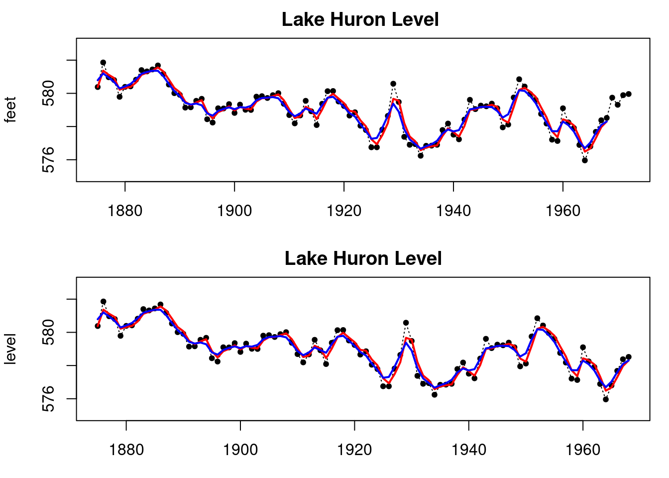
par(mfrow=c(2,1), mar = c(3, 4, 2, 1))
plot(index, LakeHuron, main = "Lake Huron Level ",type='l',
xlab="time",ylab="feet",lty=3,ylim=c(575,583))
points(index,LakeHuron,pch=20)
lines(index_filt, results_filtered$mt, type='l',
col='red',lwd=2)
lines(index_filt, results_smoothed$mnt, type='l',
col='blue',lwd=2)
# Now let's look at the DLM package
library(dlm)
model=dlmModPoly(order=1,dV=1,dW=1,m0=570,C0=1e4)
results_filtered_dlm=dlmFilter(LakeHuron[1:T],model)
results_smoothed_dlm=dlmSmooth(results_filtered_dlm)
plot(index_filt, LakeHuron[1:T], ylab = "level",
main = "Lake Huron Level",
type='l', xlab="time",lty=3,ylim=c(575,583))
points(index_filt,LakeHuron[1:T],pch=20)
lines(index_filt,results_filtered_dlm$m[-1],col='red',lwd=2)
lines(index_filt,results_smoothed_dlm$s[-1],col='blue',lwd=2)
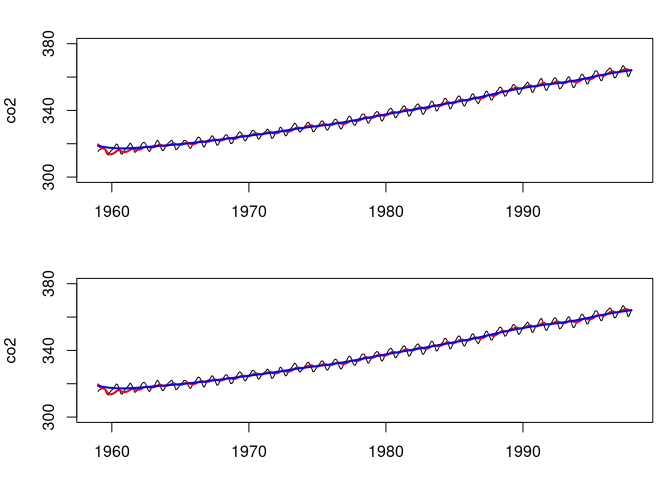
# Similarly, for the second order polynomial and the co2 data:
T=length(co2)
data=list(y_t = co2)

FF <- (as.matrix(c(1,0)))
GG <- matrix(c(1,1,0,1),ncol=2,byrow=T)
VV <- as.matrix(200)
WW <- 0.01*diag(2)
m0 <- t(as.matrix(c(320,0)))
C0 <- 10*diag(2)

## wrap up all matrices and initial values
matrices <- set_up_dlm_matrices(FF,GG, VV, WW)
initial_states <- set_up_initial_states(m0, C0)

## filtering and smoothing
results_filtered <- forward_filter(data, matrices,
                                   initial_states)
results_smoothed <- backward_smoothing(data, matrices,
                                       results_filtered)
#### Now, using the DLM package:
model=dlmModPoly(order=2,dV=200,dW=0.01*rep(1,2),
                 m0=c(320,0),C0=10*diag(2))
# filtering and smoothing
results_filtered_dlm=dlmFilter(data$y_t,model)
results_smoothed_dlm=dlmSmooth(results_filtered_dlm)

par(mfrow=c(2,1), mar = c(3, 4, 2, 1))
plot(as.vector(time(co2)),co2,type='l',xlab="time",
     ylim=c(300,380))
lines(as.vector(time(co2)),results_filtered$mt[,1],
      col='red',lwd=2)
lines(as.vector(time(co2)),results_smoothed$mnt[,1],
      col='blue',lwd=2)

plot(as.vector(time(co2)),co2,type='l',xlab="time",
     ylim=c(300,380))
lines(as.vector(time(co2)),results_filtered_dlm$m[-1,1],
      col='red',lwd=2)
lines(as.vector(time(co2)),results_smoothed_dlm$s[-1,1],
      col='blue',lwd=2)
```