1.1 Rules of Probability, Odds & Expectation
- Background reading: This reviews the rules of probability, odds, and expectation.
For all its discussion of different paradigms of probability, the course lacks a rigorous definition of probability.
Definition 1.1 (Sample Space and Sample Point)
\Omega = \{ \forall w \mid w \text { is an outcome of an experiment} \} \ne \emptyset \tag{1.1}
then \Omega is called a sample space.
Since
\Omega \ne \emptyset \implies \exists\ \omega \in \Omega \tag{1.2}
then \omega is called a sample point
Definition 1.2 (Event)
\Omega \ne \emptyset \implies \exists \mathcal{F} \subset 2^\Omega \implies \exists A\in F \tag{1.3}
Let \mathcal{F} denote a family of subsets of a sample space \Omega, and A any such subset. Then A is called an event
Definition 1.3 (Elementary Event) An event composed of a single point \omega is called an elementary event.
Definition 1.4 (Outcome) We say that event A happened if when conducting the experiment we got an outcome \omega and \omega\in A.
Definition 1.5 (Certain Event) \Omega is called the certain event.
Definition 1.6 (Impossible Event) \emptyset is called the impossible event.
Definition 1.7 (σ-Algebra) A family of events \mathcal{F} with the following properties:
\Omega is the universal set
\Omega \in \mathcal{F} \tag{1.4}
\mathcal{F} is closed under complement operation:
\forall A \in \mathcal{F} \implies A^c \in \mathcal{F} \tag{1.5}
\mathcal{F} is closed under countable unions:
\exists A_i \in \mathcal{F} \quad i \in \mathcal{N} \implies \bigcup_{n=1}^\infty {A_i} \in \mathcal{F} \tag{1.6}
is called a \sigma-algebra or a \sigma-field .
some properties of \sigma-algebra
- https://math.stackexchange.com/questions/1330649/difference-between-topology-and-sigma-algebra-axioms
- An epsilon of room: pages from year three of a mathematical blog § 2.7
Definition 1.8 (Probability Measure) if \Omega is a sample space Definition 1.1 and \mathcal{F} a \sigma-algebra Definition 1.7 for \Omega then a function P: \mathcal{f} \to [0,1] with the following properties:
Total measure of the sample space is 1: \mathbb{P}r(\Omega)=1 \tag{1.7}
countably additive for pairwise disjoint countable collections of events: is called a probability measure over \mathcal{F}. \forall E_{ i \in \mathbb{N} } \quad \mathbb{P}r(\bigcup_{n\in \mathbb{N} }{E_n})=\sum_{n\in \mathbb{N} } \mathbb{P}r(E_n) \tag{1.8}
then P is a probability measure over \mathcal{F}
Definition 1.9 (Probability Space) If \Omega is a sample space Definition 1.1 and \mathcal{F} a \sigma-algebra Definition 1.7 for \Omega, and P a probability measure (Definition 1.8) for \mathcal{F} then the ordered set <\Omega,\mathcal{F},P > is called a probability space
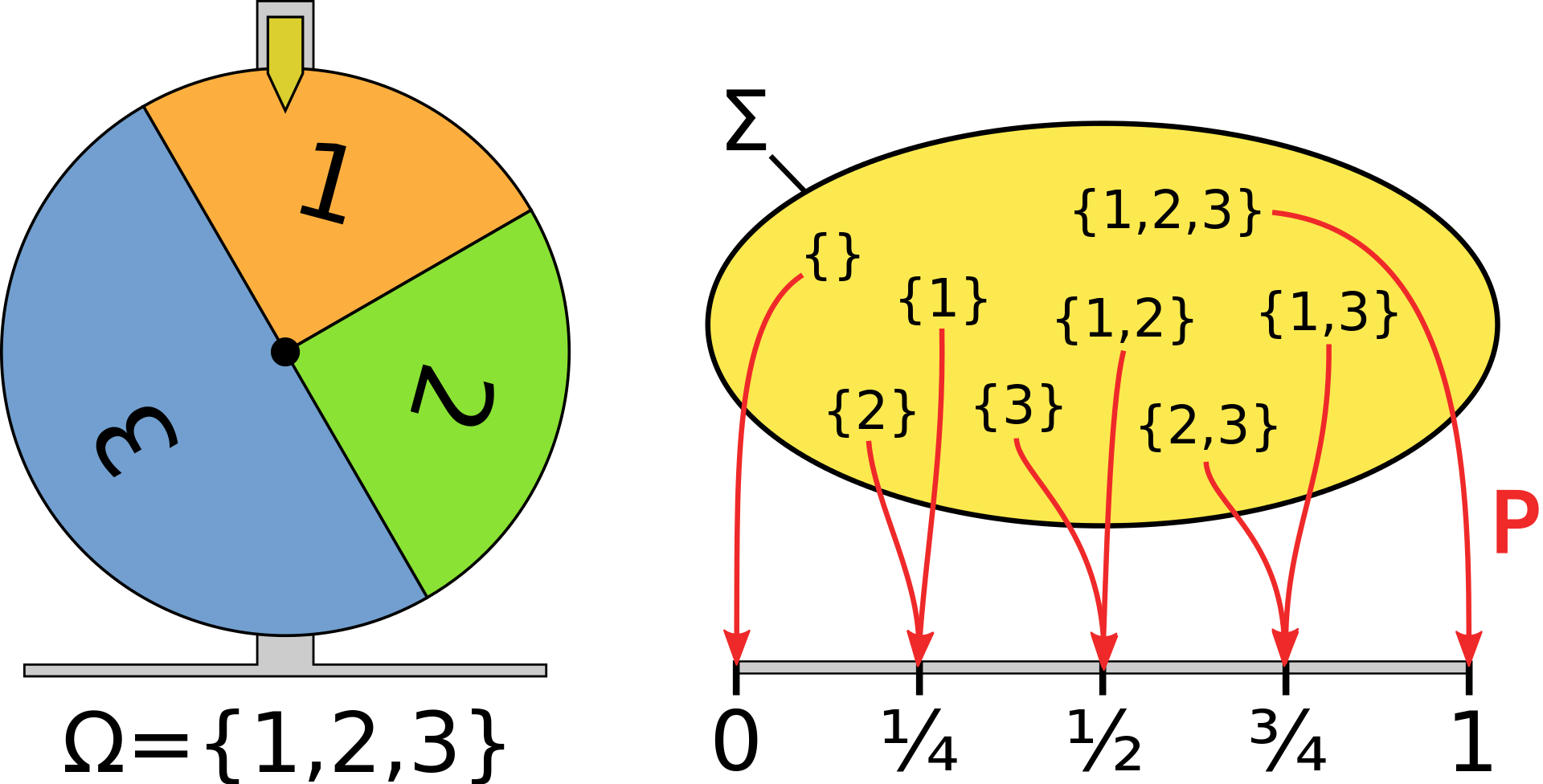
sometimes \mathcal{F} is replaced with \Sigma. for the \sigma-algebra like in the figure below
1.2 Properties of Probability Measures
The probability of the null event is 0.
\mathbb{P}r(\emptyset) = 0 \tag{1.9}
Probabilities of all possible events (the space of all possible outcomes) must sum to one.
\mathbb{P}r(\Omega) = 1 \tag{1.10}
A\cap B = \emptyset \implies \mathbb{P}r(A \cup B) = \mathbb{P}r(A)+\mathbb{P}r(B) \tag{1.11}
\mathbb{P}r(A^c) =1-\mathbb{P}r(A) \qquad \forall A\in\Omega \tag{1.12}
if A is an event in \Omega then A^C is in Omega and since they are mutually exclusive by Equation 1.10
If S is the certain event in class C \Omega then
For every event X in class \Omega
1 \ge \mathbb{P}r(X) \ge 0 \qquad \forall X \in \Omega \qquad \text{(P1)} \qquad \tag{1.13}
Probabilities add to one:
\sum_{i\in \Omega} \mathbb{P}r(X=i)=1 \qquad \text{(P2)}\qquad \tag{1.14}
The complement of an event A is A^c
\mathbb{P}r(S) = 1 \tag{1.15}
If events A_\lambda are mutually exclusive (only one event may happen):
\mathbb{P}r(A_1 \cup A_2) = \mathbb{P}r(A_1) + \mathbb{P}r(A_2) - \mathbb{P}r(A_1\cap A_1) \tag{1.16}
\mathbb{P}r(\bigcup_{\lambda\in \Omega} A_\lambda)=\sum_{\lambda \in \Omega} \mathbb{P}r(A_\lambda) \tag{1.17}
if {B_i} is a finite or countably infinite partition of a sample space \Omega then
\mathbb{P}r(A) = {\sum_{i=1}^{N} \mathbb{P}r(A \cap B_i)}= {\sum_{i=1}^{N} \mathbb{P}r(A|B_i)\mathbb{P}r(B_i)} \tag{1.18}
1.2.1 Odds
C-3PO: Sir, the possibility of successfully navigating an asteroid field is approximately 3,720 to 1!
Han Solo: Never tell me the odds! — Star Wars Episode V: The Empire Strikes Back
Another way to think about probabilities is using odds Equation 1.19. Odds are more intuitive when we are thinking about the risk of an event happening or not happening. and when we consider the risk associated with uncertainty odds are a handy way of considering the risks.
Definition 1.10 (Odds Definitions) the odds of an event A are:
\mathcal{O}(A) = \frac{\mathbb{P}r(A)}{\mathbb{P}r(A^c)} = \frac{ \mathbb{P}r(A)}{1-\mathbb{P}r(A)} \tag{1.19}
It is also possible to convert odds to probabilities Equation 1.20
Theorem 1.1 (Probability from odds) \mathbb{P}r(A) = \frac{ \mathcal{O}(A)} {1+ \mathcal{O}(A)} \tag{1.20}
Proof. \begin{aligned} & & \mathcal{O}(A) &= \frac{\mathbb{P}r(A)}{1-\mathbb{P}r(A)} && \text{(odds definition)} \\ &\implies & \mathbb{P}r(A) &= \mathcal{O}(A) (1-\mathbb{P}r(A)) && (\times \text{ denominator}) \\ &\implies & \mathbb{P}r(A) &= \mathcal{O}(A) - \mathcal{O}(A) \mathbb{P}r(A) && \text{(expand)} \\ &\implies & \mathbb{P}r(A)(1+ \mathcal{O}(A)) &= \mathcal{O}(A) && \text{(collect)} \\ &\implies & \mathbb{P}r(A) &= \frac{ \mathcal{O}(A)} {1+ \mathcal{O}(A)} && \blacksquare \end{aligned}
If we are at the races and thinking about each horse a horse what we may care about is if it will win or lose. In such a case the odds can summarize the ratio of past successes and failures to win. Odds seem to be in line with a frequentist view summarizing ratios of success to failure. In reality, the other horses have odds as well and we may want to consider the probability of winning given the other horses in the race, and perhaps other parameters, like the track type, length of the race, jockey, and perhaps some hot tips. So let us not get ahead of ourselves
Many of these formulas are rather tedious. But, once you start to work on a data science project you will often discover that there are some problems with the data and because of that you cannot use your favorite algorithm. Or worse when you do the results are not very useful. It is at this point that the ability to think back to first principles will be very fruitful. The more of this material you can recall, the more the dots will connect, and your ability will translate into models of increasing sophistication. Luckily, the rules of probability are logical. So it is fairly easy to remember or even derive if you take some time to understand them.
I realize that figuring out which results are more useful is easier in hindsight. And one of the reasons I am taking these courses is to annotate in my note the results I think to be most useful.
1.2.2 Expectation
The expectation of a random variable (RV) X is the weighted average of the outcomes it can take weighted by their probabilities.
Definition 1.11 (Expectation for a discrete RV) \mathbb{E}(x) = \sum^N_{i=1} x_i \times \mathbb{P}r(X=x_i) \tag{1.21}
Definition 1.12 (Expectation for a continuous RV) \mathbb{E}(x) = \int_{\Omega} x \mathbb{P}r(X=x) dx \tag{1.22}
1.3 Probability Paradigms
We start by looking at probability as defined or interpreted under three paradigms. Probability is at its root a logical and scientific approach to formalizing and modeling uncertainty.
The three paradigms are:
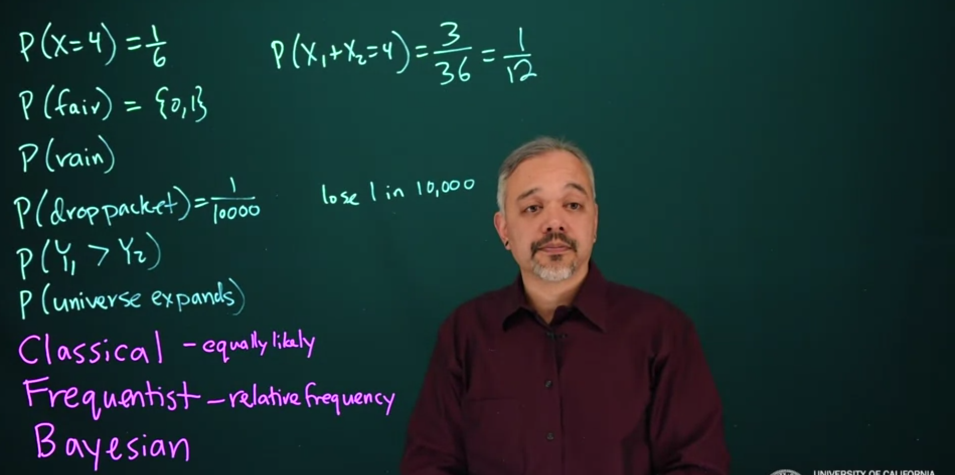
Definition 1.13 (Classical Probability) Deals primarily with cases where probabilities are distributed equally, like with dice and cards.
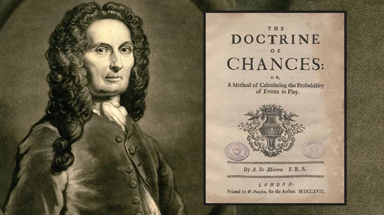
The Probability of an Event is greater or less, according to the number of chances by which it may happen, compared with the whole number of chances by which it may either happen or fail. — (Moivre 1718)
Abraham de Moivre (1667-1754) was a prominent French mathematician known for his significant contributions to the field of probability and his work on the foundations of Bayesian statistics. His research and writings played a crucial role in establishing the mathematical principles of probability theory and laid the groundwork for future advancements in the field.
De Moivre is best known for his work on the theory of probability. He made significant advancements in understanding the Binomial distribution and its application to games of chance and coin tossing. In his influential book, “The Doctrine of Chances” (1718), he presented a comprehensive treatise on probability theory, providing mathematical explanations for various phenomena such as the law of large numbers and the central limit theorem. His book became a standard reference in the field and greatly influenced subsequent research on probability.
Furthermore, de Moivre’s work laid the foundation for Bayesian statistics, although the term “Bayesian” was not coined until many years after his death. He developed a formula known as de Moivre’s theorem, which establishes a connection between the normal distribution and the binomial distribution. This theorem became a fundamental tool in probability theory and enabled the calculation of probabilities for large sample sizes. It provided a bridge between frequentist and Bayesian approaches, allowing for the estimation of parameters and the quantification of uncertainty.
And thus in all cases it will be found, that although Chance produces irregularities, still the Odds will be infinitely great, that in process of Time, those Irregularities will bear no proportion to the recurrency of that Order which naturally results from Original Design. (Moivre 1718)
He was an active participant in scientific societies and maintained correspondence with renowned mathematicians of his time, including Isaac Newton and James Stirling. His work played a crucial role in disseminating mathematical knowledge and promoting the study of probability theory across Europe. De Moivre’s research and writings laid the groundwork for the development of probability theory and Bayesian statistics. His ideas and formulas continue to be foundational in the field, and his contributions have had a lasting impact on mathematics, statistics, and the broader scientific community.
His work remains an essential reference for researchers and serves as a testament to his profound understanding of probability and statistics.
Further, the same Arguments which explode the Notion of Luck, may, on the other side, be useful in some cases to establish a due comparison between Chance and Design: We may imagine Chance and Design to be, as it were, in Competition with each other, for the production of some sorts of Events, and many calculate what Probability there is, that those Events should be rather be owing to the one than to the other. (Moivre 1718)
Definition 1.14 (Frequentist Probability) Defines probabilities using long-run limits of frequencies from repeated independent sampling generated by a hypothetical infinite sequence of experiments from a population
Frequentist probability or frequentism is an interpretation of probability; it defines an event’s probability as the limit of its relative frequency in many trials AKA long-run probability. Probabilities can be found, in principle, by a repeatable objective process and are thus ideally devoid of opinion. The continued use of frequentist methods in scientific inference, however, has been called into question.
- Since in reality we cannot repeat most experiments many times.
- “by definition, scientific researchers do not possess sufficient knowledge about the relevant and irrelevant aspects of their tests and populations to be sure that their replications will be equivalent to one another” - Mark Rubin 2020
Definition 1.15 (Bayesian Probability) Defines probability starting with a subjective view of the problem called a prior and updates it as evidence comes in using Bayes Rule.
The lesson and assignments test these views with examples - but the division is rather artificial to me. Not that it does not exist, but rather different authors on the subject treat it differently.
1.4 Bayesian Probability and Coherence
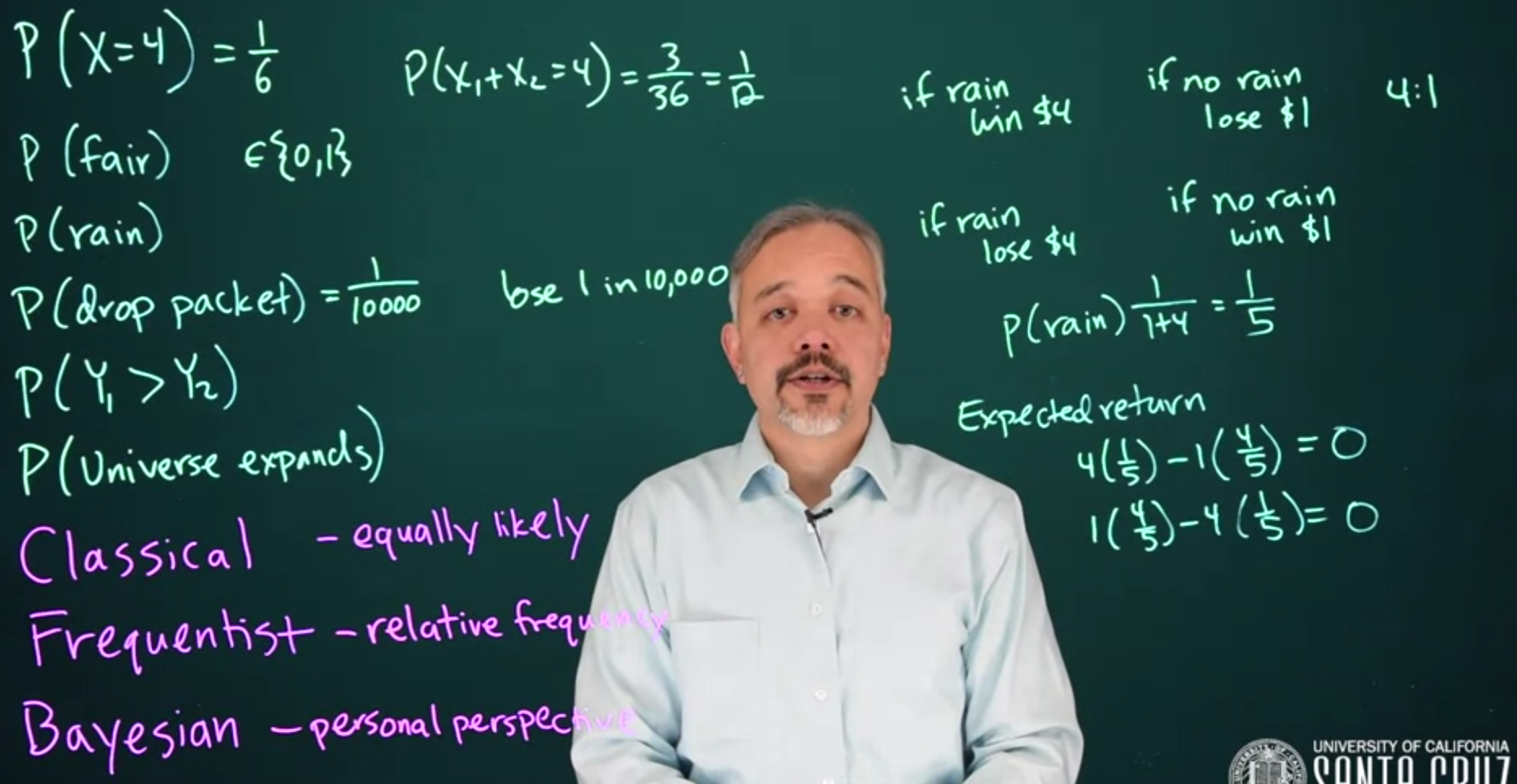
A notion of a fair bet - one which we would take either way for the same reward.
- coherence following the rules of statistics
- incoherence or Dutch book one would be guaranteed to lose money.
From the subjective standpoint, no assertion is possible without a priori opinion, but the variety of possible opinions makes problems depending on different opinions interesting.
Bruno de Finetti 1906-1985 was born in Innsbruck (Austria) to an Italian family. He studied mathematics at the University of Trieste, where he developed a keen interest in probability theory and its applications.
After completing his doctoral studies in 1928, de Finetti embarked on a distinguished academic career. His first research work dealt with mathematical biology and was published, in 1926 when he was still an undergraduate. After graduation and up to 1931, he worked in the mathematical office of the Central Italian Agency for Statistics. From 1931-46, de Finetti worked in Trieste at Assicurazioni Generali, one of the most important insurance companies in Italy. In the same period, he lectured at the University of Trieste and the University of Padua.
One of de Finetti’s most significant contributions was his development of the theory of subjective probability, also known as the Bayesian interpretation of probability. He developed his ideas independently of F. P. Ramsey who also published on this (Ramsey 1926)
In his seminal work, (Finetti 1937), he proposed that probability should be interpreted as a personal measure of belief or degree of uncertainty rather than as a frequency or long-run proportion. This subjective approach allowed for the incorporation of prior information and updating of beliefs in light of new data, forming the basis of Bayesian inference.
Probabilistic reasoning – always to be understood as subjective – merely stems from our being uncertain about something. (Finetti 2017 § preface)
It is impossible to summarize in a few paragraphs the scientific activity of de Finetti in the different fields of mathematics (probability), measure theory, analysis, geometry, mathematics of finance, economics, the social sciences, teaching, computer science, and biomathematics or to describe his generous and complex personality as a scientist and a humanitarian. De Finetti discussed his own life in a book edited by Gani (1982). See also the article by Lindley (1989).
My thesis, paradoxically, and a little provocatively, but nonetheless genuinely, is simply this :
PROBABILITY DOES NOT EXIST.
… Probability, too, if regarded as something endowed with some kind of objective existence, is no less a misleading misconception, an illusory attempt to exteriorize or materialize our true probabilistic beliefs. (Finetti 2017 § preface page x)
de Finetti was a brilliant statistician but his books and papers have garnered a reputation of being challenging to read both in the original Italian, French and English translation. The above quote embodies his radical point of view which he challenged other statisticians to rethink their views.
What I think he meant is that meant primarily was that probabilities unlike physical quantities cannot be measured in the objective sense. de Fineti was well versed with quantum mechanics, where physical quantities like the position and speed of an electron are interpreted primarily through probabilities in a wave equation, to include a discussion in the start of his second volume.
A large part of this course is that we are inferring parameters - which are often probabilities.
Another milestone result by de Finetti is his theorem
Representing uncertainty with probability: Don’t use any outside information on this question, just determine probabilities subjectively. The country of Chile is divided into 15 administrative regions. The size of the country is 756,096 square kilometers. How big do you think the region of Atacama is? Let:
- A_1 be the event: Atacama is less than 10,000 km^2.
- A_2 be the event: Atacama is between 10,000 and 50,000 km^2
- A_3 be the event: Atacama is between 50,000 and 100,000 km^2
- A_4 be the event: Atacama is more than 100,000 km^2 Assign probabilities to A_1 \ldots A_4
| Event | Min km^2 | Max km^2 | P |
|---|---|---|---|
| A_1 | 0 | 10k | \frac{1}{4} |
| A_2 | 10k | 50k | \frac{1}{4} |
| A_3 | 50k | 100k | \frac{1}{4} |
| A_4 | 100k | \frac{1}{4} |
- What do I know at this point?
- The expected area for the region is \frac{750,000}{15}=50,000\ km^2 .
- What Do I believe?
- I believe that the administrative regions have significantly different sizes
- from my familiarity with some other countries.
- As I don’t know if Atacama is large or small my best bet is to assign equal probabilities to each event.
Atacama is the fourth largest of 15 regions. Using this information, I revised my probabilities as follows:
| Event | Min km^2 | Max km^2 | P |
|---|---|---|---|
| A_1 | 10k | \frac{1}{16} | |
| A_2 | 10k | 50k | \frac{3}{16} |
| A_3 | 50k | 100k | \frac{6}{16} |
| A_4 | 100k | \frac{6}{16} |
- What do I know?
- The expected area is \frac{750,000}{15}=50,000\ km^2 .
- I know that Atacama is the Fourth largest.
- What Do I believe?
- I believe that the administrative regions have significantly different sizes - from my familiarity with some other countries.
- How do I revise my guesstimate?
- If the region sizes are equally sized I should gamble mostly on A_2 and A_3 .
- But I think there are a few large regions and many smaller ones.
- Also I know that 11 regions are smaller than Atacama and that 3 three are larger.
- None of the events can yet be ruled out.
- A_1 seems extremely unlikely as it necessitates the top three regions account for almost all of the area of the country. \frac{750,000 - 14 * 10,000}{3} = 203,333.3 that’s about 4 times the average for each state.
- A_2 is fairly unlikely to require the top three regions to account for \frac{(750,000-14*20000)}{3}=170,000 each that’s more than 3 times the average.
The smallest region is the capital region, Santiago Metropolitan, which has an area of 15,403 km^2. Using this information, I revised my probabilities as follows:
| Event | Min km^2 | Max km^2 | P |
|---|---|---|---|
| A_1 | 10k | 0 | |
| A_2 | 10k | 50k | \frac{1}{8} |
| A_3 | 50k | 100k | \frac{4}{8} |
| A_4 | 100k | \frac{3}{8} |
What do I know?
- The expected area is \frac{750,000}{15}=50,000 \quad km^2
- \mathbb{P}r(A_1)=0 since the smallest region is $ 15,403 km^2$.
- I believe that the administrative regions have significantly different sizes - from my familiarity with some other countries.
- I know that Atacama is the Fourth largest.
- If the region sizes are equally sized I should gamble mostly on A_2 and A_3.
- But I think there are a few large regions and many smaller ones.
- Also I know that 11 regions are smaller than Atacama and that 3 three are larger.
- None of the events can yet be ruled out. But A1 and A2 are now very unlikely as they would require the top three regions to account for almost all of the area of the country.
The third largest region is Aysén del General Carlos Ibáñez del Campo, which has an area of 108,494 km^2.
Using this information, I revised my probabilities as follows:
| Event | Min km^2 | Max km^2 | P |
|---|---|---|---|
| A_1 | 10K | 0 | |
| A_2 | 10k | 50K | \frac{1}{8} |
| A_3 | 50k | 100K | \frac{6}{8} |
| A_4 | 100k | \frac{1}{8} |
- The expected area is \frac{750,000}{15}=50,000 \quad km^2
- \mathbb{P}r(A1)=0 since the smallest region is $15,403 km^2 $ .
- I believe that the administrative regions have significantly different sizes - from my familiarity with some other countries.
- I know that Atacama is the Fourth largest.
- If the region sizes are equally sized I should gamble mostly on A_2 and A_3 .
- But I think there are a few large regions and many smaller ones.
- Also I know that 11 regions are smaller than Atacama and that 3 three are larger.
- None of the events can yet be ruled out. But A1 and A2 are now very unlikely as they would require the top three regions to account for almost all of the area of the country.
1.5 Discussions: Objectivity
In what ways could the frequentist paradigm be considered objective? In what ways could the Bayesian paradigm be considered objective? Identify ways in which each paradigm might be considered subjective.
- Frequentist:
- The orthodox approach is statisticians should establish an objective statistical methodology and field researchers should then use it to solve their problems. This leads to following flow charts for analysis and tests without fully understanding the model and how it works. At best one makes mistakes due to misunderstanding. But we can see that there is a systematic gaming of this methodology using p-hacking, multiple hypotheses, and hiding failed experiments leading to the publication of outrageously good results, which then cannot be replicated.
- The analysis is done on data that is supposedly sampled from a population. But the same data may belong to different populations (the city, the country, etc) each with different statistics. We should assume the same long-run frequencies would converge to different to each one of these statistics if we repeat the experiment enough times.
- The sample size, or how long we run the experiment is a tricky decision to make in advance and without prior knowledge. And if we do not decide in advance, but periodically as the data comes in. It turns out that this can completely change the outcomes of the experiment - even if both approaches have the same data.
- The choice of H_0 and H_1 is often subjective and each hypothesis can lead to yet another.
- The choice of the confidence level 95%, 99%, etc. used for statistical significance is subjective.
- If an effect size is considered large is subjective and depends on the field one studies.
- Bayesian:
- the prior should be highly informative and therefore subjective. But it can be
- uninformative and hence more objective.
- it can be difficult to decide what impact the prior should have on the posterior. Ideally, we can quantify the effective sample size for the prior data and we can understand how much information each contributes to the posterior.
1.6 Expected values
The expectation of an RV is a measure of its central tendency.
The expected value, also known as the expectation or mean, of a random variable X is denoted \mathbb{E}[X]. It is the weighted average of all values X could take, weighted by their probabilities.
I looked this up and found the following answer, see Autolatry (2015).
The RV X is a function whereas the Expectation is a Functional (a mapping from a function to a number). Mathematicians adopt the use of square brackets for functionals.
See Wikipedia contributors (2023) for more information on what a Functional is.
1.6.1 Expectation of a discrete random variable
If X is a discrete-valued random variable then its expectation is defined by(Equation 1.23)
\mathbb{E}[X]=\sum^N_{i=1} x_i \cdot \mathbb{P}r(X=x_i) = \sum^N_{i=1} x_i \cdot f(x) \tag{1.23}
where f(x) is the probability mass function (PMF) of X.
1.6.2 Expectation of a continuous random variable
If X is a continuous random variable then its expectation is defined by(Equation 1.24)
\mathbb{E}[X]=\int_{-\infty}^{\infty} x \cdot f(x) dx \tag{1.24}
while the mean is an important descriptive statistic for central tendencies, we often prefer the median which is robust to outliers, and pick the mode as a representative if we need a value in the data set.
1.6.3 Properties of Expectation
Sum and integral are linear operators so the Expectation is also a linear operator
\mathbb{E}[c]= c \tag{1.25}
\mathbb{E}[aX+bY] = a\mathbb{E}[X] + b\mathbb{E}[Y] \tag{1.26}
\mathbb{E}[g[X]] = \int{g(x)f(x)dx} \tag{1.27}
where g[X] is a function of the random variable X.
If X & Y are independent
\mathbb{E}[XY] = \mathbb{E}[X] \mathbb{E}[Y] \tag{1.28}
1.7 Variance
Variance is the dispersion of a distribution about the mean.
Definition 1.16 For a discrete random variable, the Variance is defined using (Equation 1.29)
\mathbb{V}ar(X)=\sum^N_{i=1} (x_i-\mu)^2 \mathbb{P}r(X=x_i) \tag{1.29}
Definition 1.17 For a continuous random variable, the Variance is defined using (Equation 1.30)
\mathbb{V}ar[X]=\int_{- \infty}^{\infty} (x-\mu)^2 f(x)dx \tag{1.30}
1.7.1 Properties of Variance
\mathbb{V}ar[c] = 0 \tag{1.31}
if X and Y are independent then
\mathbb{V}ar[aX+by] = a^2\mathbb{V}ar[X] +b^2\mathbb{V}ar[Y] \tag{1.32}
otherwise
\mathbb{V}ar[aX+by] = a^2\mathbb{V}ar[X] +b^2\mathbb{V}ar[Y] + 2ab\mathbb{C}ov(X,Y) \tag{1.33}
where \mathbb{C}ov(X,Y) is the covariance of X and Y.
Here is one of the most useful identities (Equation 1.34) for wrangling with variance using the expectation of X and X^2.
\begin{aligned} \mathbb{V}ar[X] &= \mathbb{E}[(X- \mathbb{E}[X])^2] \\&= \mathbb{E}[X^2] − (\mathbb{E}[X])^2 \end{aligned} \tag{1.34}
1.8 Covariance
Covariance is a measure of the joint variability of two random variables. It indicates the direction of the linear relationship between the variables.
If X and Y are two random variables, the covariance of X and Y is defined as:
\begin{aligned} \mathrm{Cov}(X,Y) &= \mathbb{E}[(X-\mathbb{E}[X])(Y-\mathbb{E}[Y])] \\ &= \mathbb{E}[XY]-\mathbb{E}[X]\mathbb{E}[Y] \end{aligned} \tag{1.35}
1.9 Correlation
Correlation is a standardized measure of the linear relationship between two random variables. It is a dimensionless quantity that ranges from -1 to 1.
The correlation coefficient \rho_{XY} is defined as the covariance of X and Y divided by the product of their standard deviations:
\rho_{XY} = \frac{\mathrm{Cov}(X,Y)}{\sigma_X\sigma_Y} \tag{1.36}