75.1 Classification with Mixture Models 🎥

Classification is a supervised learning problem where we want to predict the class of a new observation based on its features.

According to the instructor the main difference from clustering is that in classification we have a training set. I would think the main difference is that we have labels for some of the data, while in clustering we do not have labels at all.

The fact that we have labels and a training set means we should know how many classes we have and we can use these labels to train a model and use it to predict the class of a new observation.

The instructor mentions Support Vector Machines (SVM), logistic regression and linear discriminant analysis (LDA) as familiar examples of classification methods. These and a number of others are covered in (James et al. 2013). We will focus on Naïve Bayes classifiers as it is the most similar to mixture models and the EM algorithm which we have seen earlier

75.2 Mixture Models and Naïve Bayes classifiers 🎥

75.3 Naïve Bayes classifiers {sec-naïve-bayes-classifiers}

The idea of Naïve Bayes classifiers is that we want to know what is the probability that observation i belongs to class k and we can obtain this using Bayes’ theorem by computing the prior probability that an observation is in that class. This is just the frequency of the class multiplied by the density of that class and divided by the sum over the classes of the same expression.

\mathbb{P}r(x_i \in \text{class}_k) = \frac{w_k \cdot g_k(x_i \mid \theta_k)}{\sum_{j=1}^K w_j \cdot g_j(x_i\mid \theta_j)} \tag{75.1}

where w_k is the prior probability of class k, g_k(x_i \mid \theta_k) is the density of class k, and \theta_k is the parameter of class k.

with

\tilde{c}_i = \arg \max_k \mathbb{P}r(x_i \in \text{class}_k)\ for \; i=n+1,\ldots,n+m \tag{75.2}

The naïve Bayes classifier assumes that the features are conditionally independent given the class. This means that the density of class k can be written as the product of the densities of each feature given the class: g_k(x_i\mid \theta_k) = \prod_{l=1}^p g_{kl}(x_{il}\mid\theta_{kl}) \tag{75.3}

where g_{kl}(x_{il} \mid \theta_{kl}) is the density of feature l given class k and \theta_{kl} is the parameter of feature l given class k. This means that we can estimate the density of each feature separately and then multiply them together to get the density of the class.

This is a very strong assumption and is not true in general. However, it works well in practice and is often used in text classification problems where the features are the words in the text.

The Naïve Bayes classifier is a special case of the mixture model where the components are the classes and the densities are the product of the densities of each feature given the class. This means that we can use the EM algorithm to estimate the parameters of the model in the same way as we did for the mixture model. The only difference is that we need to estimate the densities of each feature separately and then multiply them together to get the density of the class.

Video Transcript

The last class of problems for which mixture models are very useful is classification problems. If you come from the machine learning literature, you will call this supervised classification to contrast, again, unsupervised classification that I called clustering before. The goal in supervised classification is to start with a training set and use the information in a training set to determine the classes or the labels of a second group of observations that you call the test set. So you start with a training set that contains known labels classes. You also have a test set that has unknown labels, and you want to use this information to make predictions about the test set labels. For example, you may want to decide whether a person suffers from a disease or not based on a set of medical tests, maybe P medical tests, and you have gone out and measured those tests in a number of individuals. So you know those individuals whether they are sick or they are not sick. Based on that training set that is labeled where you know what the real quality of the individuals is, then you go out and you are going to pick just a random person that comes into your medical appointment, and based on the results of the test, now you want to decide if that individual suffers from the disease or not. So the presence of the training set is really what distinguishes clustering problems from classification problems. In clustering problems, we don’t have a training set. We don’t have anything that gives us a hint about how the classes look like. We’re trying to do the process of dividing the observations into groups in some sense blindly. That’s why it’s sometimes called unsupervised classification because you can think that the training set provides supervision in how you do the classification. In typical supervised classification problems on the other hand, you do have that training set. You do have that group of labeled observations that can help you make decisions about how the new groups will look like. So in some sense, supervised classification is a simpler problem than unsupervised classification because of the presence of the training set. Now, there are a number of classification procedures out there. This is a fairly common problem in the literature. You may be familiar with things like support vector machines or logistic regression for classification. I want to discuss today the similarities between using mixture models for classification and some techniques such as linear discriminant analysis, and in particular with Naïve Bayes classifiers. The idea of Naïve Bayes classifiers is very simple. So if you want to know what is the probability that observation i belongs to class k, you can typically obtain that by just using Bayes’ theorem by computing the prior probability that an observation is in that class. That is typically just the frequency of the class multiplied by the density of that class and divided by the sum over the classes of the same expression. Now, again, this should be very familiar. This quantity here is essentially what we used both in the EM algorithm to compute the [inaudible] case and in the MCMC algorithm if you are fitting a mixture model from a Bayesian perspective to sample the class labels C sub x. So in other words, it’s clear just from writing the expression from Naïve Bayes that there should be a very close relationship between doing Naïve Bayes and doing mixture models. In fact, you can cast Naïve Bayes classifiers as just as a special case of mixture models. Let’s discuss Naïve Bayes classifiers where we use Gaussian kernels for the classification. Let’s enter this a little bit of notation. So remember that we have both a test set and a training set. So let’s call X_1 up to X_n my training set, and let’s call X_n plus 1 up to X_n plus m the test set. In other words, we have n observations in the training set, we have m observations in the test set and we just group the observations together so that the first n in the sample are the training and last m are the test. In addition to this, because the training set is labeled, we’re going to have C_1 up to C_n are known, but C_1 or C_n plus 1 up to C_m plus n are unknown and we want to protect them. Let’s write a Naïve Bayes classifier that uses Gaussian kernels, and we’re going to use the more general Gaussian kernels that we can. So in that case, the probability that observation i belongs to class k, it’s going to be equal to Omega_k 1 over the square root 2 Pi to the p. Remember that we’re working with P variate normal. So we can have P features for each individual, determinant of Sigma_k to the minus one 1/2 X of minus one 1/2 X_i minus Mu k transpose sigma sub k inverse X_i minus Mu k, divided by the sum over the components of exactly the same expression. This has to be l, minus Mu sub l transpose sigma l inverse X_i minus Mu l. So this is just Bayes theorem as we have written multiple times in this course. So what you do is, you need this expression only for the training set because for the test set you already know what class you are in. So what you typically do is a two-step process in which you get Mu k hat and Sigma hat sub k are estimated from the training set. You could do different things, but it’s very fairly common to just fit a multivariate Gaussian to each one of the components. So your Cs, your labels divide your training set into groups. For each one of those groups, you fit one different normal and that gives you Sigma and Mu. Similarly, for Omega k, you want to get an estimate for Omega k, and the natural thing to do is to just use the frequency, the fraction of the observations in the training set that belong to each one of the classes. Once you have those, then you classify new observations as by letting C_i be equal to the org max of that probability. Where the probabilities are computed by plugging in these maximum likelihood estimators in this formula up here. As I said, this is done for n plus 1 all the way to n plus m. So you don’t need to do this for the training set, the training set you know the labels and you use those labels to compute the MLEs that get plugged into this. Now, with additional observations in those MLEs, you can decide what are the classes for them. So this is what a naïve Bayes classifier based on Gaussian distributions for each one of the classes would look like. Now, this is exactly the same as the EM algorithm that we have discussed in the past for mixture models, if we make a couple of assumptions or if we incorporate a couple of assumptions into the algorithm. So let’s write down that next. We can recast the algorithms that we just saw for naïve Bayes classifier based on Gaussian kernels in the context of the EM algorithm that we have been discussing for mixtures. That is very easy, we’re going to think, again, about an E-step and an M-step, and we’re going to add an additional post-processing step, if you will. In our E-step, if you remember, what we did in the past was to compute the indicators for the variables. So that is our variables V_i,k that corresponds to the weights that are associated with each one of the components. What we’re going to do in this case is we’re going to define the V_i,k in a very simple fashion rather than doing it using Bayes theorem. Because we actually know what observations or what components are generating each of the observations in the training set, we can call V_i,k just one or zero if C_i is equal to k and zero otherwise, for all the observations that go from one to n. In other words, this is for the training set. Once we have defined our E-step in this way, we’re going to have an M-step where we compute Mu sub k and Omega sub k. To put it in the same way that we did with the EM algorithm, this is going to have a very particular shape. It’s going to have the sum from one to n of V_i,k X_i divided by the sum from one to n of V_i,k. In a similar expression for my matrix Sigma, Sigma is going to be Sigma sub k, it’s going to be one over the sum of the V_i,k from one to n, sum from one to n of V_i,k X_i minus Mu k, X_i minus Mu k transpose. These are expressions that we have seen in the past when filling mixtures of multivariate Gaussians to data. This is just a fancy way, so casting it in terms of the E-step and the M-step, it’s just a fancy way to say, I know what my assignments are, for sure, because this is a training set. So this is just computing the average of the observations that are in category K because, in this case, these are either zeros or ones. Similarly, here, this is just the variance covariance matrix of the observations that are in component K, but it’s written in a fancy way using this V_i,k as indicators. Then, we have a post-processing. It’s in the post-processing step where the test set comes into play. So for now, we have only used the training set for our calculations. In the post-processing step, what we do is we allocate C_i based on the arc max over K of the posterior distribution of the class allocations. So that is probability that X_i belongs to class K. So this is just another way to write the algorithms as we had before, that is very simple in the context of [inaudible]. So why did I go through the trouble of expressing this in this complicated manner when I had a very simple description before? Well, because now you can try to generalize this from this supervised setting where you completely break apart the estimation of the parameters that only uses the training set and the classification that only uses the test set. You can actually try to combine information from both, and it should be clear that if you have training sets that are just very small compared to the test set, the estimates that you get for Mu and Sigma will be very bad because they will be based on very few observations, very few data points. So if you could somehow use some of the information that you are recovering by doing the classification to help you estimate what Mu and Sigma are, they’ll probably give you more robust, stronger algorithm. How to do that should be relatively straightforward once you think about it in this context. For the observations to the training set, we have the value of the V_i,k, but we could add an estimate of the value of the V_i,k for the observations in the test set to this calculation. We already know how to do that. So we’re going to turn the algorithm iterative now. So these guys are always going to be defined in this way because I know the C’s, but these guys are refined at every iteration of the algorithm. I’ll just make this essentially equal to the probability that X_i belongs to class K given the current parameters of the model, so given the current Omegas, the current Mus, and the current Sigmas. Then, I can extend my sums to m down here and down here. Now, what I’m doing is, for the observations that I know what class they are in, these weights are either zeros or ones. For the ones that I don’t know but I’m trying to classify, they will be some number between zero and one, and I’m just going to do a weighted average so you can think about this, again, as a weighted average of the information that I know for sure, and the information that I’m recovering about Mu and Sigma from the classification. So again, this now becomes an iterative algorithm, so I need to think about t plus 1, t plus 1, t plus 1, t plus 1, t plus 1, t plus 1, and t plus 1. So I have turned what was just a two-step algorithm that doesn’t require any iteration, I turned it into an iterative algorithm that uses the whole sample to estimate the parameters of the classes. This is sometimes called a semi-supervised; I don’t necessarily like the term very much. But this is sometimes called a semi-supervised algorithm, in the sense that it’s not completely supervised because of the addition of this information and the fact that now, the sums go up to m. But it’s also not fully unsupervised because I’m using the information, I’m using this piece up here that has information where I know their true labels. Once the algorithm converges, I’m still going to do the post-processing step that is to go from this V_i,k’s that I computed here for the test set to generate what are the labels for those observations.

75.3.1 LDA and the EM algorithm 🎥

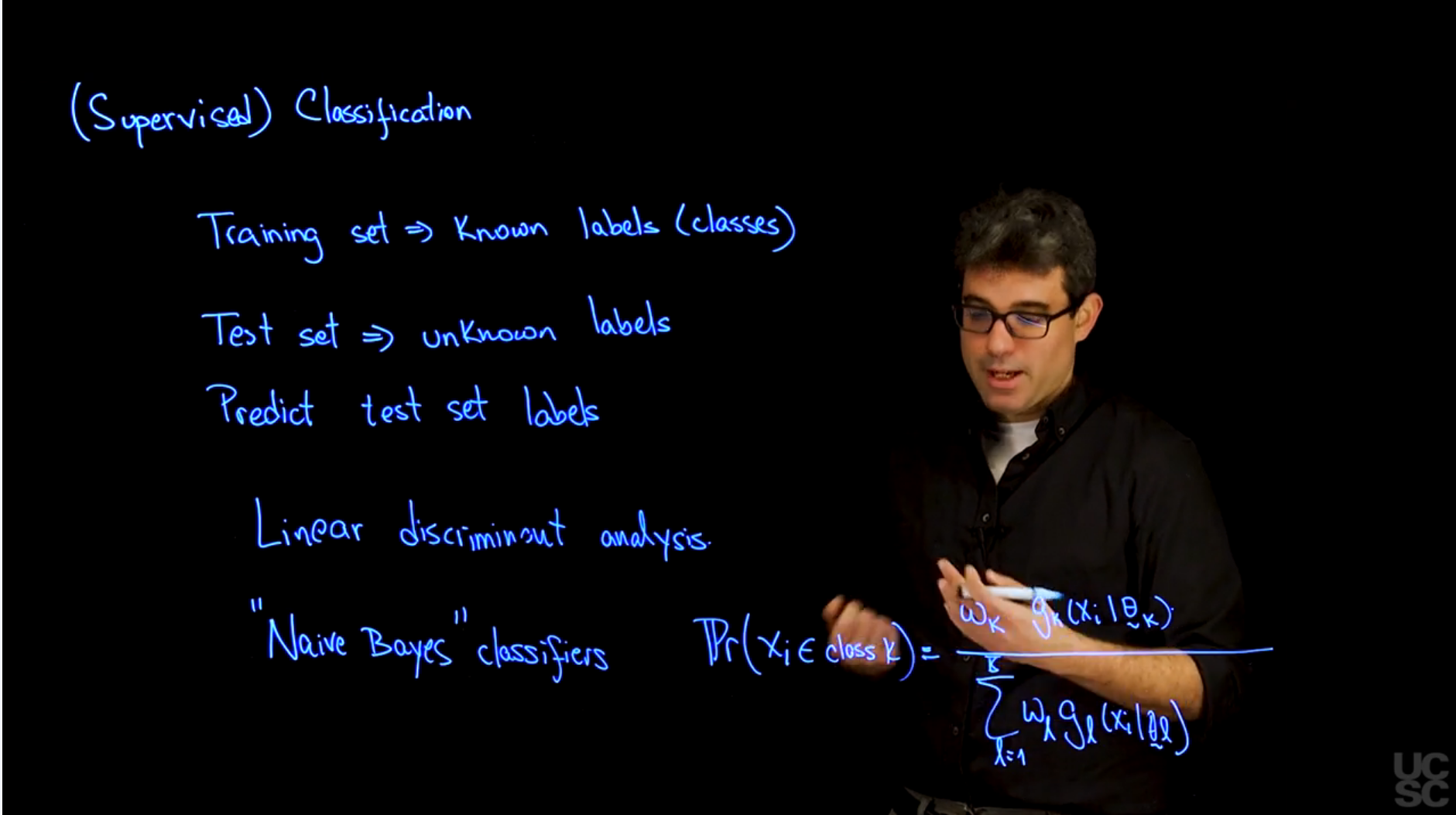
It is important to understand the connection between using mixture models for classification and other procedures that are commonly used out there for classification. One example of those procedures that has a strong connection is linear discriminant analysis and also to quadratic discriminant analysis.

To illustrate that connection, we start with a very simple mixture model.

So let’s start with a mixture model of the form:

f(x) = \sum_{k=1}^2 \omega_k \frac{1}{\sqrt{2\pi}} \frac{1}{\sqrt{\text{det}(\Sigma)}} e^{-\frac{1}{2}(x - \mu_k)^T \Sigma^{-1} (x - \mu_k)}. \tag{75.4}

Video Transcript

And to illustrate that connection, let’s start with a very simple mixture model.

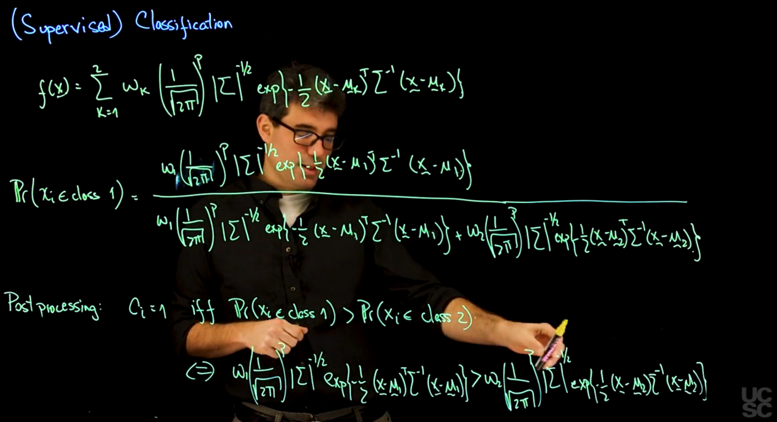
So let’s start with a mixture model of the form, f(x) = the sum from 1 to 2. So I’m going to be working only with two components of omega k, 1 over the square root 2pi to the p determinant of sigma to the -1 half, x- 1 half, x, mu sub k, transpose sigma inverse, x- mu sub k. So this is two-component mixture with locations bearing with a component, but the same variance-covariance matrix for the two components that I have in the mixture.

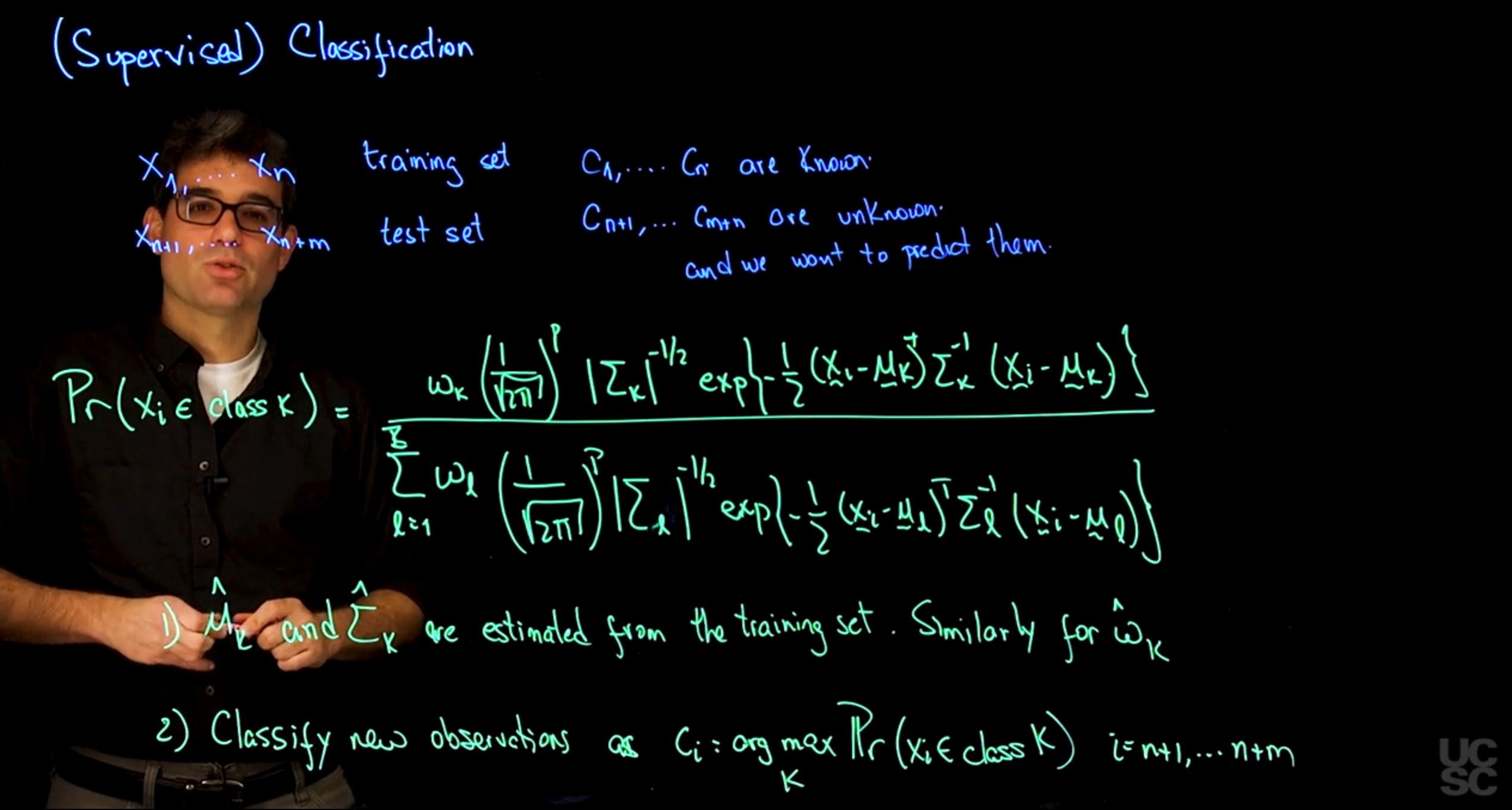
And let’s think about how the procedure would look like if we were to do Naïve Bayes classification using this mixture. If I follow the unsupervised example that I have discussed before, the probability that I put observation i in class, 1, say, I only have two classes.

So as you see again, consider one of them and the other one is just 1- the numbers that I get here. It’s going to be equal.

And I’m going to expand this in all its glory. It’s going to be a little bit long. So it’s going to be omega 1, 1 over the square root 2pi to the p determinant of sigma to the- 1 half, x of- 1 half, x- mu k transpose sigma inverse x- mu k. And in the denominator, we’re going to have the same expression first. And then we’re going to have omega 2, that is just 1- omega 1 but 2pi to the p determinant of sigma to the- 1 half x- 1 half x- mu 2, sigma inverse x- mu 2. Okay, and we know that the probability that xi belongs to class 1 is exactly the same expression but replacing mu, 1 which is what should be up here, replacing mu1 with mu2.

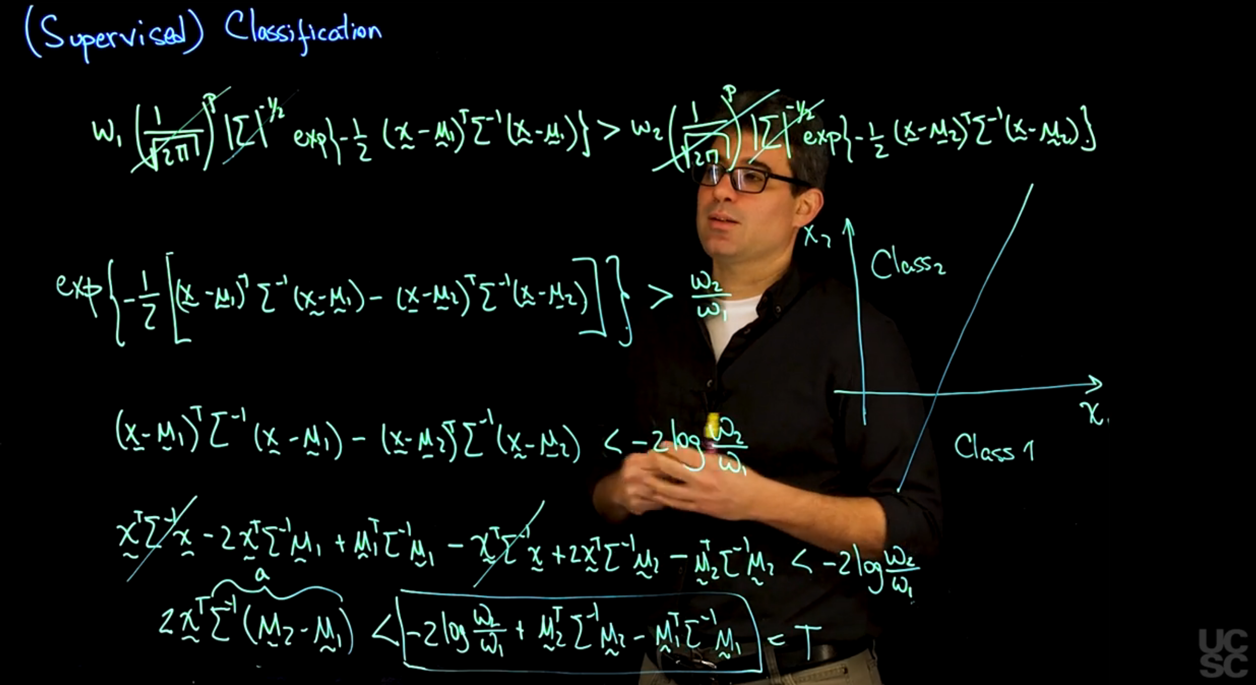
So, in the post processing step, we are going to assign C sub i = 1 if and only if the probability that xi belongs to class 1 is greater than the probability that xi belongs to class 2. And because the two expressions are the same in the denominator, the only thing that changes is the numerator, then this happens if and only if omega 1, 1 over the square root 2pi to the p determinant sigma to the- 1 half x- 1 half, X- mu1 transpose sigma inverse x- mu1, Is greater than omega 2, 1 over the square root 2pi to the p determinant of sigma to the- 1 half x of- 1 half x- mu2, sigma inverse x- mu2. So probability of class 1 greater than probability of class 2 only if this quantity is greater than the same thing but evaluated for the second component in the mixture. So let’s do a little bit of algebra and let’s try to simplify this expression a little bit and we will see that that simplification leads to a very nice expression that matches exactly what you get out of linear discriminant analysis. So now we want to simplify this expression that corresponds to the situation where we’re going to label an observation coming from class 1, and we want to make it much more compact. So a few things that we can observe. So one of them is we have 1 over square root 2pi to the p on both sides, so we can cancel that. The other thing that we observe is that we have the determinant of the variance-covariance matrix on both sides. And because we’re assuming that the two components have the same variance- covariance matrix, we can again just simplify both terms on either side. And the next thing that I’m going to do is I’m going to move all the omegas to one side and bring all the terms with the exponentials to the other side. If I do that, I’m going to end up on the left hand side with the exponent of- 1 half, X- mu1 transpose sigma inverse x- mu1. And then this term came to the other side in the denominator, but that just means that when it goes into the exponential, I need to change all to reverse signs. So it’s going to be- x- mu2 transpose sigma inverse x- mu2. So that’s the expression once you move this to the denominator and combine the two exponentials. And this needs to be greater than omega 2 divided by omega 1. Now, some further simplifications. I can take the logarithm on both sides and I can multiply by -2 on both sides, and I end up with an expression that looks like x- mu 1 transpose sigma inverse x- mu1- x- mu 2 transpose sigma inverse x- mu 2 has to be less than, because I’m going to end up multiplying by a -2. So less than -2 log of omega 2 divided by omega 1. So now we have this difference of two quadratic forms needs to be less than a certain constant that depends on what are my prior weights for each one of the two components. Now, to finish simplifying this, we need to expand these two squares, which is pretty straightforward. So first we’re going to have x sigma inverse x transpose sigma inverse x. This is just a square. So it’s going to be 2 times x transpose sigma inverse mu1. And finally, \mu_1 transpose sigma inverse \mu_1. And then we need to subtract a similar expression but using mu2 for it turns. So it’s going to be x transpose sigma inverse x. It’s going to be +, in this case, 2x transpose sigma inverse mu2. And finally, again,- mu2 transpose sigma inverse mu2, and all of these needs to be less than -2 log of omega 2, Divided by omega 1. So you can see that the expressions are relatively straightforward.

And one of the things that is very nice, and it’s a consequence of having the same variance-covariance matrix for each one of the components, is that now this quadratic term of the data is going to cancel out. And so, we can just basically learn together a couple of terms. So we can write, 2 times, X transpose sigma inverse multiplied by mu2- mu1. So I’m taking this term and combining it with this term. So, the term here and the term here.

And then I’m going to say that this has to be less than -2 times log of omega 2 divided by omega 1, and I’m going to move this two terms to the right. So,+ mu2 transpose sigma inverse mu2- mu1 transpose sigma inverse mu1. So this is actually quite a bit of simplification and it’s a very interesting one. Because you can think about this, Thing on the right hand side, just call this T for threshold. So this is your sum threshold and that threshold is basically computed based on the training data. So if I know the classes of some observations, I can get what the means for each one of the classes are, I can estimate the common sigma, and I can estimate the relative frequencies. And with that, I can obtain a stress score from the training set. And I can think about this matrix product as sum vector a. The form of this simplified expression is very interesting. You can see that the right-hand side, all this expression in the box, it’s just a threshold that can be easily computed from the training set. We can estimate the weight and we can estimate the mean and the covariance of the two components. And then, this product of the variance-covariance or the inverse of the variance-covariance matrix times the difference of the means corresponds to a vector a that can also be computed from the training set. So essentially, the decision of whether we classify an observation in class 1 or class 2 is going to depend on whether a linear combination, and that’s what x transpose times a is, is just a linear combination of the values of x. So whether this linear combination of the values of x is greater than a given threshold or not. In other words, what we’re doing, In a setting where we only have two variables, for example, x1 and x2, the linear combination of the entries is just a line on the plane. So this product just corresponds to a line. And by deciding whether we are above the line or below the line, we’re just saying that one of the regions corresponds to class, 2, and the other region corresponds to class 1. So this is the reason why the procedure is called linear discriminant analysis because it uses a straight line to decide whether observations should be classified in class 1 and class 2. Now, there are some more interesting things that you can do.

For example, you don’t have to assume that the sigmas are the same, you could assume that the \sigma_i are different. If you were to do that, then you’d be in a situation that is analogous to this one with the main difference being that now these terms here wouldn’t necessarily simplify.

But then, you can rearrange terms in such a way that now, you’re going to have a quadratic form of x being less than a certain threshold. And in that case, you’re separating hyperplane.

Instead of being a hyperplane or line, it’s going to be a quadratic form. And that is the reason why when you’re doing Naïve Bayes and you’re working with kernels that are Gaussian and have different variance-covariance matrices, you call the procedure quadratic discriminant analysis. Because it uses a quadratic form, a parabola or something like that to separate the two classes that you’re working with.

The nice thing about thinking about this classification procedures in the context of mixture models is again, thinking about ways in which you can generalize and address the shortcomings of the procedure. It’s clear that the main issue with classification procedures based on Gaussians is that data in the real world sometimes doesn’t look like multivariate Gaussian distributions.

One possible extension is to instead of considering the density, this ps here to be a single Gaussian, you can kind of use mixtures a second time and borrow some ideas from when we did density estimation. And say well, I’m going to have a mixture and each component of that mixture is in turn a second mixture that may have a few components. And that may allow for the shape of the clusters to be much more general, and that’s what we call mixture discriminant analysis.

As before, if you instead of doing the Algorithm and the simple maximum likelihood estimation that I described before, you instead use Bayesian estimators for your process, then you will have Bayesian equivalent of linear discriminant analysis and quadratic discriminant analysis. So it is very useful to think about your statistical methods in the context of mixture models for the purpose of both generalizing and understanding the shortcomings of what you’re doing.

75.4 Linear and quadratic discriminant analysis in the context of Mixture Models 🎥

75.4.1 Classification example

This video walks through the code in Section 75.5.

Video Transcript

I’m going to illustrate now to use of mixture models for classification using the wind dataset. Unlike the previous datasets that we work with, this one is not included in R by default. So the two files that you need wind training and wind tests are available on the website, make sure that you download them and that you have them in the right directory for R to read them. And in this case, I made sure that I change the directory where I’m looking at before I start working with this, and that I put my files in there.

Okay, so the wind dataset is an interesting one, it’s a series of measurements for different varieties of wine. They come from three different cultivars, and for each particular variety of wine. They did a chemical analysis and measure 13 different variables that have to do with different chemical components present in the world. So we have a label set where we know which samples from which of the three cultivars. And now we want to use the information that we clean out of that to classify to decide a series of new wines to assign them to the cultivar that we think they come from. We actually do know the truth for the test set, so we will actually first do the predictions we’ll act as if we don’t know what the cultivar of the test set is. And then we will compare the predictions that we’re making against the truth, as a way to tell how well the algorithm is to it, okay. So the first thing that we need to do is load our dataset as I said, you need to make sure that the two files are in the directory where you’re working. So make sure of that, remember that we called n the sample size of the training set and m the training size the size of the test set. So I’m just calling the variables that way, and I’m going to use mixture of normals mixture of multivariate normals by location and scale. So I’m going to use a method that is essentially equivalent to doing quadratic discriminant analysis. And, I want to run the Algorithm that I discussed on the board, but in a situation which we assume that we’re going to work with semi-supervised learning. In other words, I went around the Version of the algorithm in which we’re going to use all the observation both in the training and the test set, to learn the parameters of the classes. So it’s going to be an iterative algorithm. So we know in advance as we have three classes because we have three cultivars. B in this case is going to be 13 because there are 13 features that were measured on each wine. So if you come down here, you can see that B 13, we can try to do a graph of the data. In this case the graph is not going to be terribly readable because there are so many variables, but it may still provide a little bit of intuition. So the variables that are measured things like alcohol, the ash, the alkalinity, the level of magnesium, the hue that has to do with how dark the wine is, proline. So you can see here where the variables are there are measured, and even though the graph is not very readable at least you can see that the classes do not fully overlap. So we do have some hope that we may be able to do classification in the problem. That’s pretty much the main thing that you can say out of this graph here, okay. So, as I said before mixture of models with different components, different variances and different means for each component its normal component in the mixture. Same type of standard initialization that we have done before. And we’re going to do the E and the M step here, remember that for the observations in the training set. We know the class, so the value of B are either 0 or 1, and because we do the calculation first in the log scale, then we do either 0 or minus infinity. So 0 corresponds to probability of 1 and minus infinity corresponds to a probability of 0 in the log scale. And then for the observations in the test set, we have just a regular way in which we compute the probability that the observation comes from each class. And once we have done this then we subtract, we do as we have always done subtract maximums and then re-standardize. So this is how the ES step gets adapted in the case of semisupervised classification. And then the structure of the m-step is exactly the same structure of the regular Algorithm. So we compute means and variances for each one of the components as weighted averages of the different quantities. We check conversions in the standard way, in which we have been checking convergence. And finally once everything is done, we will get a classification, so let’s run it for this dataset. It runs actually quite quickly, we have only 12 iterations and we have converged. Now what the Algorithm gives gave us is just the B values, that is the probability that an observation comes from a given class. Now, we typically are going to want to convert those peas into Cs and as we saw on the board, that is done by just selecting the class that has the highest probability.

So if we do that for our training set in this case, and if you look at the indexes here, they run from n + 1 to n + m, which means that we’re looking at test set. If we just get what is the maximum we can see that the first block of observations is assigned to component two. Most of this block is assigned to component two except for this guy here, and then the the remaining block of observation is assigned to components three. So now how does that compare with the truth? So we can actually go into winder test, and the first column of that file contains the true labels, and we can say that it matches actually pretty well. So the ones all match, the twos match except for one guy, the one we had kind of identified before, and the threes all match together. And we can actually if you just want to have a summary of how many errors you make. You can do a little comparison like this, and you can find that there is only a single error in the classification that the algorithm does.

Now let’s compare that with just using quadratic discriminant analysis and linear discriminant analysis. The way they are implemented in R, so QDA and LDA are the two functions that you will need, they are part of the mass package. So, We first feed the QDA model and then we that fitted model to predict the classes. And now if we see what the regular QDA does is it’s going to give me this long list of probabilities for the test set. And we can turn those into labels and in particular we can see how many errors we’re making in the prediction. And you can see that we make a single mistake, which is actually not the mistake that we had made before. So if we just look at this one here and we compare it against the, Classification that our algorithm did, and we compared it against the truth.

We see that our algorithm makes a mistake in this observation and QDA does not, and instead the error is somewhere else in this sample. It’s basically here, so you can see that the QDA classifies this as two, when the reality is that it’s a three. So our results are not identical to QDA even though our method is asymptotically going to be equivalent to QDA but they don’t give us exactly the same result, but they give us very similar accuracy. Interestingly if you run LDA and you try to look at how many errors you have in that case, you will see that LDA in this case has no errors, even though it’s a simpler more restrictive classification procedure. So this can happen, so it’s a relatively large sample, so a single a difference in a single error is not a very large difference. So, hopefully this illustrates how classification or how measurements can be used for classification in a real life setting.

75.5 Sample EM algorithm for classification problems 🗒️ \mathcal{R}

In the following code sample we will illustrate how to use the EM algorithm for classification problems.

Using mixture models for classification in the wine dataset Compare linear and quadratic discriminant analysis and a (semi-supervised) location and scale mixture model with K normals Comparing only against the EM algorithm

76 Semi-supervised, quadratic discriminant analysis

library(MASS)
library(mvtnorm)
wine.training = read.table("data/wine_training.txt", sep=",", header=TRUE)
wine.test = read.table("data/wine_test.txt", sep=",", header=TRUE)

# Set up global variables
n = dim(wine.training)[1]
m = dim(wine.test)[1]
x = rbind(as.matrix(wine.training[,-1]), 
          as.matrix(wine.test[,-1]))
p       = dim(x)[2]
KK      = 3
epsilon = 0.00001

1: Load necessary libraries
2: Load the wine dataset
3: Size of the training set
4: Size of the test set
5: The dataset stacking: training set + test set
6: Number of features in the dataset

par(mfrow=c(1,1))
par(mar=c(2,2,2,2)+0.1)
colscale = c("black","red","blue")
pairs(wine.training[,-1], col=colscale[wine.training[,1]], pch=wine.training[,1])

7: Pair plot of the training set of the wine dataset

Figure 76.1: Pair plot of the training set of the wine dataset

## Initialization step
set.seed(63252)
w   = rep(1,KK)/KK
mu  = rmvnorm(KK, apply(x,2,mean), var(x))

Sigma      = array(0, dim=c(KK,p,p))
Sigma[1,,] = var(x)/KK  
Sigma[2,,] = var(x)/KK
Sigma[3,,] = var(x)/KK

sw     = FALSE
KL     = -Inf
KL.out = NULL
s      = 0

while(!sw){
  ## E step
  v = array(0, dim=c(n+m,KK))
  for(k in 1:KK){  
    # Compute the log of the weights
    v[1:n,k] = ifelse(wine.training[,1]==k,0,-Inf)  # Training set
    v[(n+1):(n+m),k] = log(w[k]) + mvtnorm::dmvnorm(x[(n+1):(n+m),], mu[k,], Sigma[k,,],log=TRUE)  # Test set
  }
  for(i in 1:(n+m)){
    v[i,] = exp(v[i,] - max(v[i,]))/
            sum(exp(v[i,] - max(v[i,])))  
    # Go from logs to actual weights in a numerically stable manner
  }
  
  ## M step
  w = apply(v,2,mean)
  mu = matrix(0, nrow=KK, ncol=p)
  for(k in 1:KK){
    for(i in 1:(n+m)){
      mu[k,]    = mu[k,] + v[i,k]*x[i,]
    }
    mu[k,] = mu[k,]/sum(v[,k])
  }
  Sigma = array(0,dim=c(KK,p,p))
  for(k in 1:KK){
    for(i in 1:(n+m)){
      Sigma[k,,] = Sigma[k,,] + v[i,k]*(x[i,] - 
                   mu[k,])%*%t(x[i,] - mu[k,])
    }
    Sigma[k,,] = Sigma[k,,]/sum(v[,k])
  }

  # Convergence Check step
  KLn = 0
  for(i in 1:(n+m)){
    for(k in 1:KK){
      KLn = KLn + v[i,k]*(log(w[k]) + 
            mvtnorm::dmvnorm(x[i,],mu[k,],Sigma[k,,],log=TRUE))
    }
  }
  if(abs(KLn-KL)/abs(KLn)<epsilon){
    sw=TRUE
  }
  KL = KLn
  KL.out = c(KL.out, KL)
  s = s + 1
  print(paste(s, KLn))
}

8: Set the random seed for reproducibility
9: Initialize set equal weights to each component
10: Cluster centers randomly spread over the support of the data
11: Initial variances are assumed to be the same
12: Init Convergence flag to False
13: Compute the Kullback-Leibler divergence
14: If converged, set the flag to True and exit the outer loop
15: Report iteration and Kullback-Leibler divergence

[1] "1 -3146.58419305226"
[1] "2 -2942.48222029706"
[1] "3 -2873.76499310479"
[1] "4 -2852.76768638231"
[1] "5 -2796.247735428"
[1] "6 -2791.29098585679"
[1] "7 -2791.23059641487"
[1] "8 -2791.14094416728"
[1] "9 -2791.05612416221"
[1] "10 -2790.99254414223"
[1] "11 -2790.95228067601"
[1] "12 -2790.92945838389"

Next we perform predictions and evaluate the classification.

apply(v, 1, which.max)[(n+1):(n+m)]
wine.test[,1]
apply(v, 1, which.max)[(n+1):(n+m)] == wine.test[,1]
sum(!(apply(v, 1, which.max)[(n+1):(n+m)] == wine.test[,1]))

16: Predicted labels for the test set
17: True labels for the test set
18: Comparison of predicted labels with true labels
19: Number of errors in the classification - One error

 [1] 1 1 1 1 1 1 1 1 1 1 1 1 1 1 1 2 2 2 1 2 2 2 2 2 2 2 2 2 3 3 3 3 3 3 3 3 3 3
[39] 3 3 3 3 3 3 3 3
 [1] 1 1 1 1 1 1 1 1 1 1 1 1 1 1 1 2 2 2 2 2 2 2 2 2 2 2 2 2 3 3 3 3 3 3 3 3 3 3
[39] 3 3 3 3 3 3 3 3
 [1]  TRUE  TRUE  TRUE  TRUE  TRUE  TRUE  TRUE  TRUE  TRUE  TRUE  TRUE  TRUE
[13]  TRUE  TRUE  TRUE  TRUE  TRUE  TRUE FALSE  TRUE  TRUE  TRUE  TRUE  TRUE
[25]  TRUE  TRUE  TRUE  TRUE  TRUE  TRUE  TRUE  TRUE  TRUE  TRUE  TRUE  TRUE
[37]  TRUE  TRUE  TRUE  TRUE  TRUE  TRUE  TRUE  TRUE  TRUE  TRUE
[1] 1

Using the qda and lda functions in R

First we preform quadratic discriminant analysis using the qda function in R, which is part of the MASS package.

# qda
modqda = qda(grouping=wine.training[,1], x=wine.training[,-1], method="mle")
ccpredqda = predict(modqda,newdata=wine.test[,-1])
sum(!(ccpredqda$class == wine.test[,1])) # One error

[1] 1

Next we perform linear discriminant analysis using the lda function in R, which is also part of the MASS package.

modlda = lda(grouping=wine.training[,1], x=wine.training[,-1], method="mle")
ccpredlda = predict(modlda,newdata=wine.test[,-1])
sum(!(ccpredlda$class == wine.test[,1])) # No errors!!!

[1] 0