---
title : 'Determining the number of components - M5L9'
subtitle : 'Bayesian Statistics: Mixture Models'
categories:
- Bayesian Statistics
keywords:
- Mixture Models
- Maximum Likelihood Estimation
- BIC
- Bayesian Information Criteria
- Multimodality
- Numerical Instability
- notes
---
So far we considered the number of components in the mixture model as a known and fixed parameter. However, in practice, the number of components is often unknown and needs to be estimated from the data. We will cover two approaches to estimate the number of components in a mixture model:
1. **Bayesian Information Criteria (BIC)**: A model selection criterion that penalizes the likelihood of the model based on the number of parameters.
2. **Bayesian approach**: A probabilistic approach that estimates the number of components based on the posterior distribution of the model parameters.
## Bayesian Information Criteria - BIC :movie_camera: {#sec-mixtures-BIC}
{#fig-slide03-BIC .column-margin width="53mm"}
{#fig-slide04-BIC .column-margin width="53mm"}
We can consider the choice of the number of components in a mixture model as a model selection problem. In this context, we have a collection of J models, each with a different number of components. The goal is to select the model that best fits with the evidence/data while avoiding overfitting.
\index{model selection}
\index{model selection!BIC}
\index{Bayesian Information Criteria}
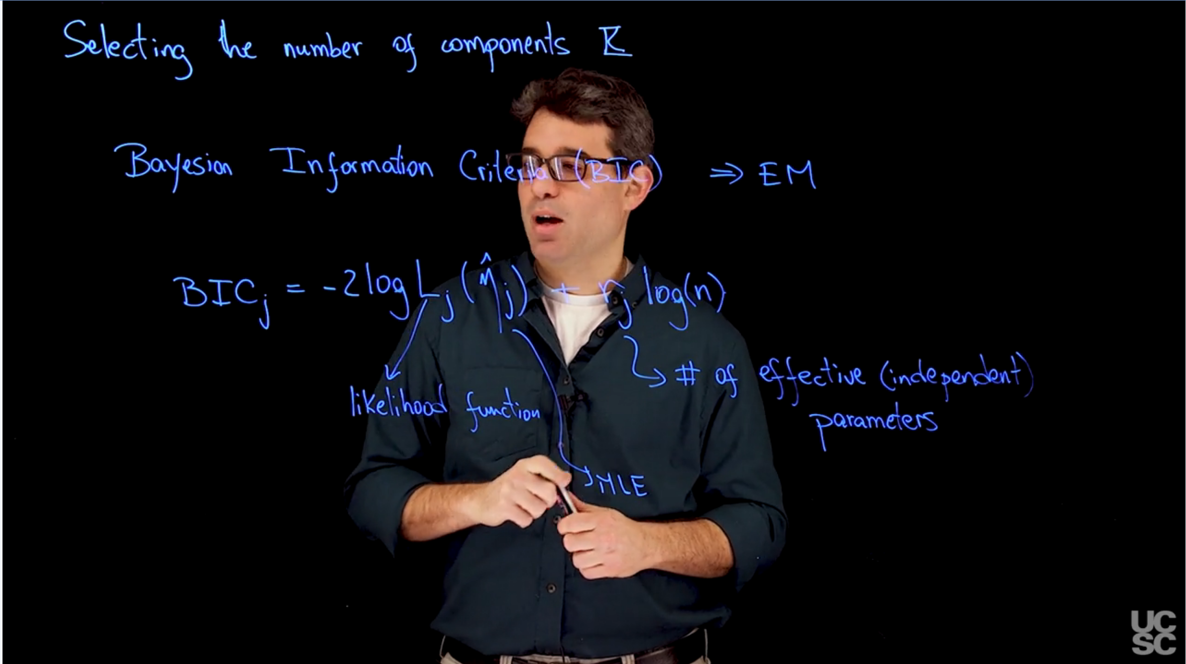
A common approach to model selection that is useful for mixture models is the Bayesian Information Criteria (BIC). Given a collection of J models to be compared, the BIC for model j is given by the formula:
$$
BIC_k = - 2\log L_j(\hat{\eta}) - r_k \log (n) \qquad
$$ {#eq-bayesian-information-criteria}
where $L_j$ is the likelihood of the model, $\hat{\eta}$ is the maximum likelihood estimate of the parameters, $r_j$ is the number of effective (independent) parameters in model j, and n is the number of observations. The model with the lowest BIC value is considered the best model.
We can interpret the first term in [@eq-bayesian-information-criteria] as a measure of the goodness of fit of the model, while the second term penalizes the model for its complexity. The BIC is a trade-off between the goodness of fit and the complexity of the model.
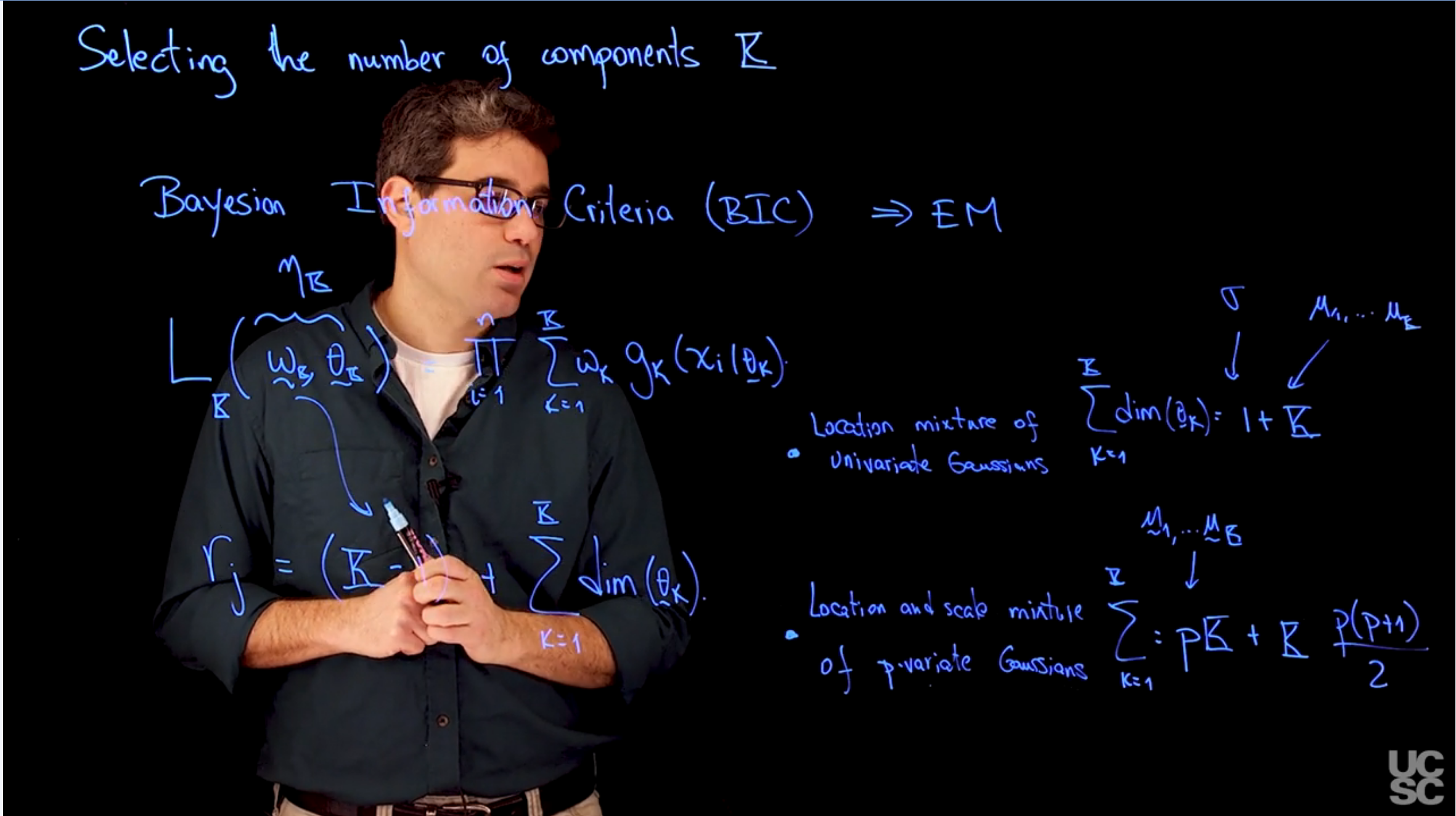
In the case of mixture models, j corresponds to the number of components K in the model. and $\eta_k$ corresponds to the parameters of the model, which include the weights and parameters of the of the component distributions i.e. $\eta_k = (w_1,\ldots,w_k, \theta_1, \ldots \theta_K)$ . The number of effective parameters in a mixture model with K components is given by:
$$
L_k(\hat{w}_1,...\hat{w}_K, \hat{\theta}_1,...,\hat{\theta_K}) = \prod_{i=1}^n \sum_{k=1}^K \hat{w}_k g(x_i|\hat{\theta}_k)
$$
furthermore, the number of effective parameters is given by:
$$
r_k = K - 1 + \sum_{k=1}^K \dim(\theta_k)
$$
## Bayesian Information Criteria Example :movie_camera:
This is a walkthrough of the code in the next section.
## Sample code: Bayesian Information Criteria :spiral_notepad:
\index{BIC} \index{dataset!galaxies}
This code sample illustrates the use of **BIC** to estimate the number of components of a Mixture Model using the galaxies dataset
```{r}
#| label: lst-bayesian-information-criteria
#| lst-label: lst-bayesian-information-criteria
#| lst-cap: "Illustrating the use of BIC to estimate the number of components of a Mixture Model using the galaxies dataset"
## using the galaxies dataset
rm(list=ls()) # <1>
library(MASS) # <2>
data(galaxies) # <2>
x = galaxies # <3>
n = length(x) # <3>
set.seed(781209) # <4>
KKmax = 20 # <5>
BIC = rep(0, KKmax-1) # <6>
w.sum = vector("list", KKmax-1) # <7>
mu.sum = vector("list", KKmax-1) # <8>
sigma.sum = rep(0, KKmax-1) # <9>
for(KK in 2:KKmax){ # <10>
### First, compute the "Maximum Likelihood" density estimate
### associated with a location mixture of 6 Gaussian distributions
### using the EM algorithm
# <11>
w = rep(1,KK)/KK # <12>
mu = rnorm(KK, mean(x), sd(x)) # <12>
sigma = sd(x)/KK # <12>
epsilon = 0.000001 # <13>
s = 0 # <13>
sw = FALSE # <13>
KL = -Inf # <13>
KL.out = NULL # <13>
while(!sw){ # <14>
# <15>
v = array(0, dim=c(n,KK))
for(k in 1:KK){
v[,k] = log(w[k]) + dnorm(x, mu[k], sigma,log=TRUE)
}
for(i in 1:n){
v[i,] = exp(v[i,] - max(v[i,]))/sum(exp(v[i,] - max(v[i,])))
}
# <16>
w = apply(v,2,mean) # <17>
mu = rep(0, KK) # <18>
for(k in 1:KK){
for(i in 1:n){
mu[k] = mu[k] + v[i,k]*x[i] # <19>
}
mu[k] = mu[k]/sum(v[,k]) # <20>
}
# <21>
sigma = 0
for(i in 1:n){
for(k in 1:KK){
sigma = sigma + v[i,k]*(x[i] - mu[k])^2 # <22>
}
}
sigma = sqrt(sigma/sum(v)) # <23>
# <24>
KLn = 0
for(i in 1:n){
for(k in 1:KK){
KLn = KLn + v[i,k]*(log(w[k]) +
dnorm(x[i], mu[k], sigma, log=TRUE))
}
}
if(abs(KLn-KL)/abs(KLn)<epsilon){
sw=TRUE
}
KL = KLn
KL.out = c(KL.out, KL)
s = s + 1
if(s/20==floor(s/20)){
print(paste(s, KLn))
}
}
w.sum[[KK-1]] = w
mu.sum[[KK-1]] = mu
sigma.sum[KK-1] = sigma
# <25>
for(i in 1:n){
BIC[KK-1] = BIC[KK-1] - 2*log(sum(w*dnorm(x[i], mu, sigma)))
}
BIC[KK-1] = BIC[KK-1] + ((KK-1) + 1 + KK)*log(n) ### KK-1 independent weights, one variance, and KK means
}
```
1. Clear the environment
2. Loading data
3. Setting up global variables
4. Setting a random seed for reproducibility
5. Setting the maximum number of components to consider
6. Initializing the BIC vector to store the BIC values for each number of components
7. Initializing list to store the weights for each number of components
8. Initializing list to store the means for each number of components
9. Initializing vector to store the standard deviations for each number of components
10. Looping over the number of components from 2 to KKmax
11. Fitting a mixture model using the EM algorithm for each number of components
12. Initializing the parameters of the mixture model
13. Initializing the convergence criteria
14. Running the EM algorithm until convergence
15. E-step: computing the responsibilities for each component
16. M-step: updating the weights, means, and standard deviations
17. Weights are updated based on the responsibilities
18. Initializing the means for the mixture model
19. Updating the means based on the responsibilities
20. Normalizing the means
21. Computing the standard deviations
22. Updating the standard deviations based on the responsibilities
23. Normalizing the standard deviations
24. Checking convergence of the EM algorithm
25. Computing the BIC for the current number of components
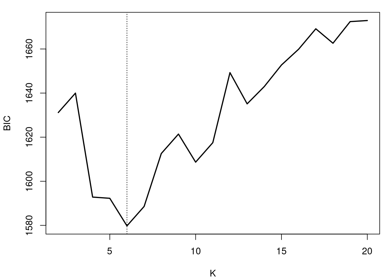
```{r}
#| label: fig-bayesian-information-criteria
#| fig-cap: "What happens with the variance (bandwidth) as K increases"
## Plot of BIC as a function of K
par(mar=c(4,4,1,1) + 0.1)
plot(seq(2,KKmax), BIC, type="l", xlab="K", ylab="BIC", lwd=2)
abline(v=6, lty=3)
```
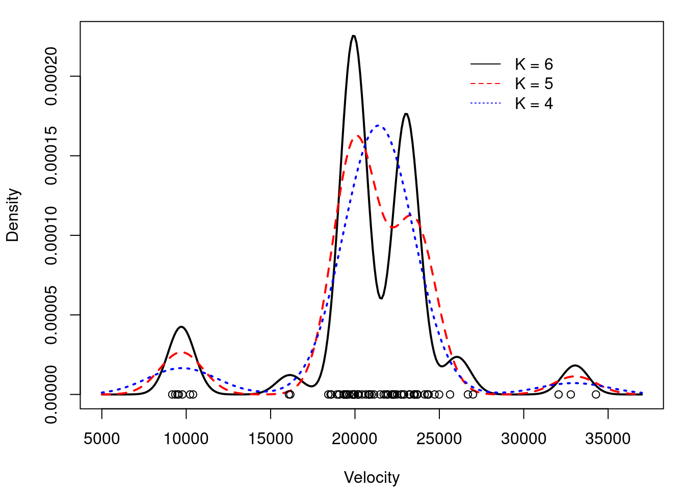
Computing density estimates for various values of K
```{r}
#| label: lst-bayesian-information-criteria-density-estimates
density.est = function(xx, w, mu, sigma){
  KK  = length(w)
  nxx = length(xx)
  density.EM = rep(0, nxx)
  for(s in 1:nxx){
    for(k in 1:KK){
      density.EM[s] = density.EM[s] + w[k]*dnorm(xx[s], mu[k], sigma)
    }
  }
  return(density.EM)
}

xx  = seq(5000,37000,length=300)
KK = 8
mdeKK8 = density.est(xx, w.sum[[KK-1]], mu.sum[[KK-1]], sigma.sum[KK-1])
KK = 7
mdeKK7 = density.est(xx, w.sum[[KK-1]], mu.sum[[KK-1]], sigma.sum[KK-1])
KK = 6
mdeKK6 = density.est(xx, w.sum[[KK-1]], mu.sum[[KK-1]], sigma.sum[KK-1])
KK = 5
mdeKK5 = density.est(xx, w.sum[[KK-1]], mu.sum[[KK-1]], sigma.sum[KK-1])
KK = 4
mdeKK4 = density.est(xx, w.sum[[KK-1]], mu.sum[[KK-1]], sigma.sum[KK-1])

## Comparing density estimates for K=4, 5 and 6
par(mar=c(4,4,1,1)+0.1)
plot(xx, mdeKK6, type="n",ylim=c(0,max(c(mdeKK4,mdeKK5,mdeKK6,mdeKK7))),
     xlab="Velocity", ylab="Density")
lines(xx, mdeKK6, col="black", lty=1, lwd=2)
lines(xx, mdeKK5, col="red", lty=2, lwd=2)
lines(xx, mdeKK4, col="blue", lty=3, lwd=2)
points(x, rep(0,n))
legend(26000, 0.00022, c("K = 6","K = 5","K = 4"),
       lty=c(1,2,3), col=c("black","red","blue"), bty="n")
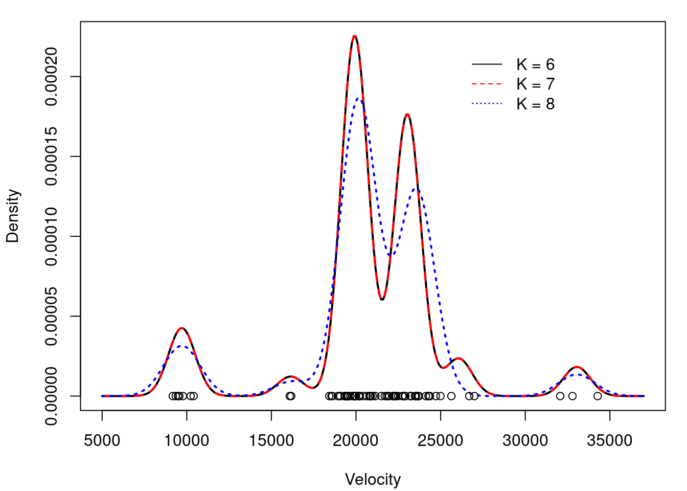
## Comparing density estimates for K=6, 7 and 8
par(mar=c(4,4,1,1)+0.1)
plot(xx, mdeKK6, type="n",ylim=c(0,max(c(mdeKK6,mdeKK7,mdeKK8))),
     xlab="Velocity", ylab="Density")
lines(xx, mdeKK6, col="black", lty=1, lwd=2)
lines(xx, mdeKK7, col="red", lty=2, lwd=2)
lines(xx, mdeKK8, col="blue", lty=3, lwd=2)
points(x, rep(0,n))
legend(26000, 0.00022, c("K = 6","K = 7","K = 8"),
       lty=c(1,2,3), col=c("black","red","blue"), bty="n")
```
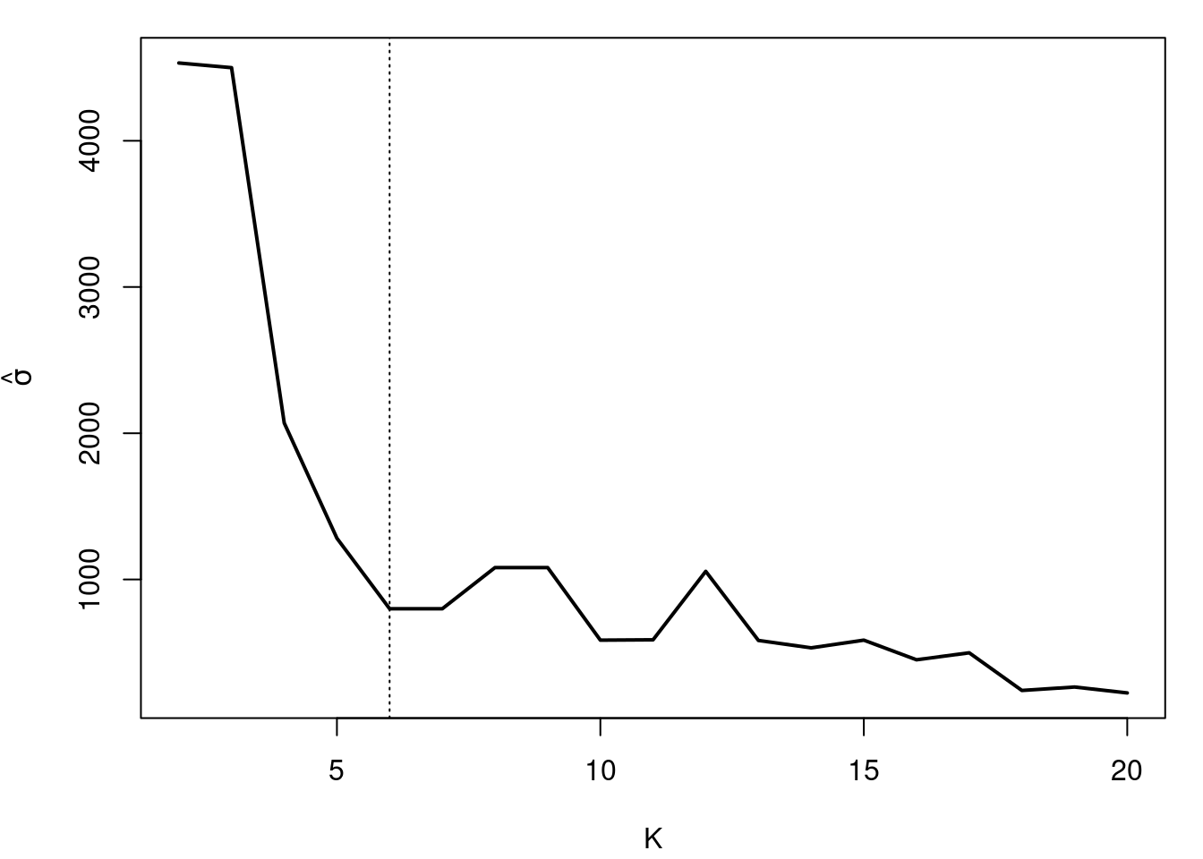
```{r}
#| label: fig-bayesian-information-criteria-variance
#| fig-cap: "What happens with the variance (bandwidth) as K increases"
par(mar=c(4,4,1,1) + 0.1)
plot(seq(2,KKmax), sigma.sum, type="l", xlab="K",
     ylab=expression(hat(sigma)), lwd=2)
abline(v=6, lty=3)
```
### Estimating the number of components in Bayesian settings :movie_camera:
[Is BIC Bayesian?]{.column-margin}
\index{Bayesian Information Criteria}
The **BIC** has the term *Bayesian* in its name, but it is not considered a Bayesian method. It is considered a frequentist method that uses the likelihood of the model and the number of parameters to estimate the number of components. In contrast, Bayesian methods use the posterior distribution of the model parameters to estimate the number of components.
\index{mixture!Dirichlet process}
So what we want is to have a posterior estimate of the number of components. We can do this by using a Dirichlet process prior on the weights of the mixture model. The Dirichlet process is a nonparametric prior that allows for an infinite number of components, but only a finite number of them will be used in the posterior distribution.
### Bayesian Information Criteria (BIC) for Mixture Models
{#fig-s05-bayesian-information-criteria-variance .column-margin width="53mm"}
{#fig-s06-bayesian-information-criteria-variance .column-margin width="53mm"}
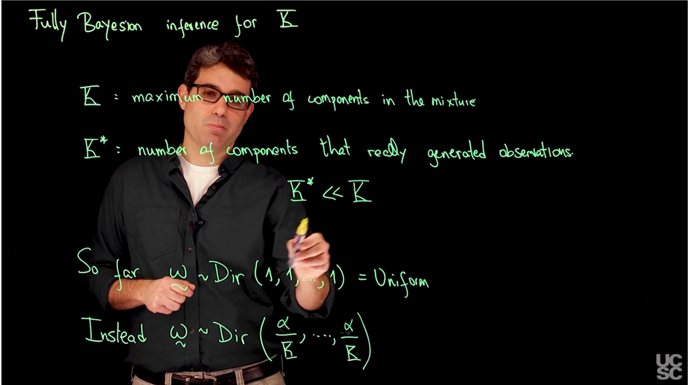
- K= maximum number of components
- K* = number of components that really generated the model
$$
K<<K*
$$
so far we used
$$
\tilde{w} \sim \mathrm{Dir}(1, \ldots ,1) = U(0,1)
$$ {#eq-dirichlet-prior-uniform}
but this won't work because the number of weights in the prior increases with K and has increasing influence on the posterior. We need to use a prior that reduces the influence on the posterior as K increase like:
$$
\tilde{w} \sim \mathrm{Dir}(\alpha/K, \ldots, \alpha/K)
$$ {#eq-dirichlet-prior-diminishing-influence}
where $\alpha$ is a hyperparameter that controls the strength of the prior. The larger the value of $\alpha$, the more influence the prior has on the posterior distribution.
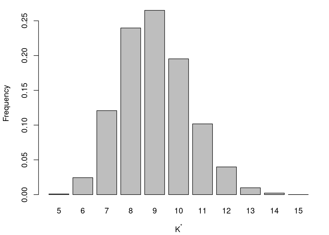
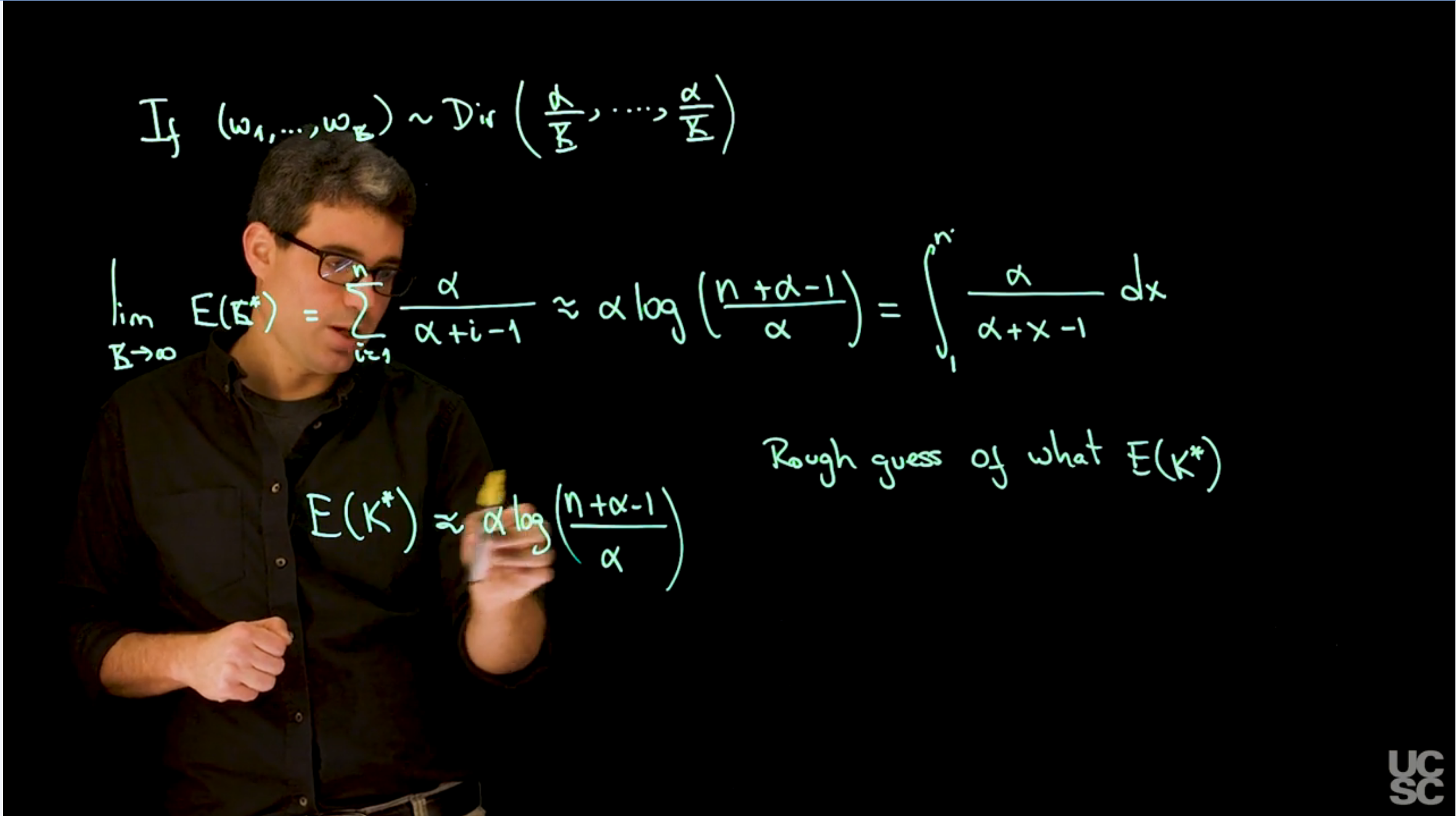
if $(w_1,\ldots,w_K) \sim \mathrm{Dir}(\alpha/K,\ldots,\alpha/K)$, then the expected number of occupied components is given by:
$$
\begin{aligned}
\lim_{K \to \infty} \mathbb{E}[K^*] &= \sum_{i=0}^n \frac{\alpha}{\alpha+i-1}
\\ & \approx \int_0^1 \frac{\alpha}{\alpha +x-1} dx \qquad \text{(Riemann sum approximation)}
\\ & = \alpha \log\left(\frac{n+\alpha-1}{\alpha}\right)
\end{aligned} \qquad
$$ {#eq-expected-number-of-occupied-components-derivation}
$$
\mathbb{E}[K^*] \approx \alpha \log\left(\frac{n+\alpha-1}{\alpha}\right)
$$ {#eq-approx-expected-number-of-occupied-components}
leaving us with just a single parameter $\alpha$ to tune. This is a very useful result because it allows us to estimate the number of components in a mixture model without having to specify the number of components in advance.
### Sample code for estimating the number of components and the partition structure in Bayesian models :spiral_notepad: {#sec-estimating-number-of-components-and-partition-structure}
```{r}
#| label: lst-estimating-number-of-components-and-partition-structure
## Full Bayesian estimation of a mixture model for density estimation in the galaxies dataset
rm(list=ls())

### Loading data and setting up global variables
library(MASS)
library(MCMCpack)
data(galaxies)
x  = galaxies
n  = length(x)
set.seed(781209)

### Fitting a Bayesian mixture model with
KK = 30   ## In this formulation, it should be interpreted as the
          ## maximum number of components allowed

## Finding the value of alpha consistent with 6 expected components a priori
ff = function(alpha)  alpha*log((82+alpha-1)/alpha) - 6
alph = uniroot(ff, c(0.01, 20))
alph$root  # 1.496393
## Priors set up using an "empirical Bayes" approach
aa  = rep(1.5/KK,KK)  # We approximate 1.496393 by 1.5
eta = mean(x)
tau = sqrt(var(x))
dd  = 2
qq  = var(x)/KK

## Initialize the parameters
w     = rep(1,KK)/KK
mu    = rnorm(KK, mean(x), sd(x))
sigma = sd(x)/KK
cc    = sample(1:KK, n, replace=T, prob=w)

## Number of iterations of the sampler
rrr   = 25000
burn  = 5000

## Storing the samples
cc.out    = array(0, dim=c(rrr, n))
w.out     = array(0, dim=c(rrr, KK))
mu.out    = array(0, dim=c(rrr, KK))
sigma.out = array(0, dim=c(rrr, KK))
logpost   = rep(0, rrr)


for(s in 1:rrr){
  # Sample the indicators
  for(i in 1:n){
    v = rep(0,KK)
    for(k in 1:KK){
      v[k] = log(w[k]) + dnorm(x[i], mu[k], sigma, log=TRUE)  #Compute the log of the weights
    }
    v = exp(v - max(v))/sum(exp(v - max(v)))
    cc[i] = sample(1:KK, 1, replace=TRUE, prob=v)
  }

  # Sample the weights
  w = as.vector(rdirichlet(1, aa + tabulate(cc, nbins=KK)))

  # Sample the means
  for(k in 1:KK){
    nk    = sum(cc==k)
    xsumk = sum(x[cc==k])
    tau2.hat = 1/(nk/sigma^2 + 1/tau^2)
    mu.hat  = tau2.hat*(xsumk/sigma^2 + eta/tau^2)
    mu[k]   = rnorm(1, mu.hat, sqrt(tau2.hat))
  }

  # Sample the variances
  dd.star = dd + n/2
  qq.star = qq + sum((x - mu[cc])^2)/2
  sigma = sqrt(1/rgamma(1, dd.star, qq.star))

  # Store samples
  cc.out[s,]   = cc
  w.out[s,]    = w
  mu.out[s,]   = mu
  sigma.out[s] = sigma
  for(i in 1:n){
    logpost[s] = logpost[s] + log(w[cc[i]]) + dnorm(x[i], mu[cc[i]], sigma, log=TRUE)
  }
  logpost[s] = logpost[s] + log(ddirichlet(w, aa))
  for(k in 1:KK){
      logpost[s] = logpost[s] + dnorm(mu[k], eta, tau, log=TRUE)
  }
  logpost[s] = logpost[s] + dgamma(1/sigma^2, dd, qq, log=TRUE) - 4*log(sigma)
  if(s/500==floor(s/500)){
    print(paste("s =",s))
  }
}
nunique = function(x)   length(unique(x))
Kstar = apply(cc.out[-seq(1,burn),],1,nunique)
par(mar=c(4,4,1,1) + 0.1)
barplot(table(Kstar)/sum(table(Kstar)), xlab=expression(K^"*"), ylab="Frequency")
#dev.print(file="postKstaralpha2.pdf", dev=pdf)
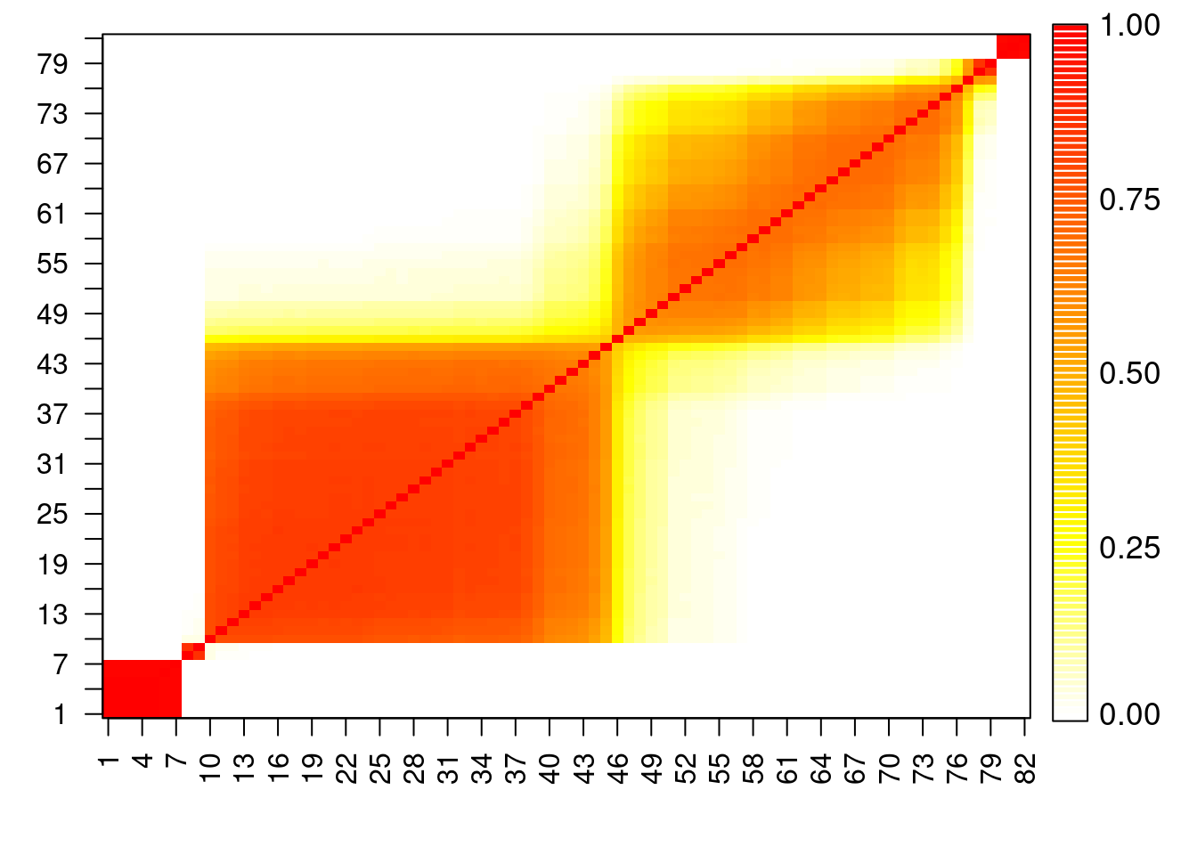
## Construct pairwise co-clustering matrix for this dataset
pairwise = matrix(0, nrow=n, ncol=n)
for(s in 1:(rrr-burn)){
for(i in 1:n){
for(j in i:n){
pairwise[i,j] = pairwise[i,j] + as.numeric(cc.out[s+burn,i]==cc.out[s+burn,j])
pairwise[j,i] = pairwise[i,j]
}
}
}
DD = pairwise/max(pairwise)
heatmapplot = function(DD, alab, subsetaxis, llc=FALSE){
n = dim(DD)[1]
#colorscale = rev(gray(0:100 / 100))
colorscale = c("white", rev(heat.colors(100)))
nf = layout(matrix(c(1,2),nrow=1,ncol=2), c(7,1), TRUE)
par(mar=c(4,3,1,0.5))
###Display heat-map
image(seq(1,n), seq(1,n), DD, axes=F, xlab="", ylab="",
col=colorscale[seq(floor(min(100*DD)), floor(max(100*DD))) + 1])
axis(1,at=subsetaxis,labels=alab[subsetaxis],las=2,cex.axis=1)
axis(2,at=subsetaxis,labels=alab[subsetaxis],las=2,cex.axis=1)
box()
abline(v = llc+0.5)
abline(h = llc+0.5)
###Display color scale
par(mar=c(3,0,0,0))
plot(1:100,1:100,xlim=c(0,2),ylim=c(0,100),type="n",axes=F,xlab ="",ylab ="")
yposr = 1:100
rect(0, yposr-.5, 0.5, yposr+.5,col = colorscale, border=F)
rect(0, .5, 0.5, 100.5,col = "transparent")
text(0.42,c(yposr[1],yposr[25],yposr[50],yposr[75],yposr[100]),c("0.00","0.25","0.50","0.75","1.00"),pos=4,cex=1.1)
}
heatmapplot(DD, seq(1,n), seq(1,n,by=3))
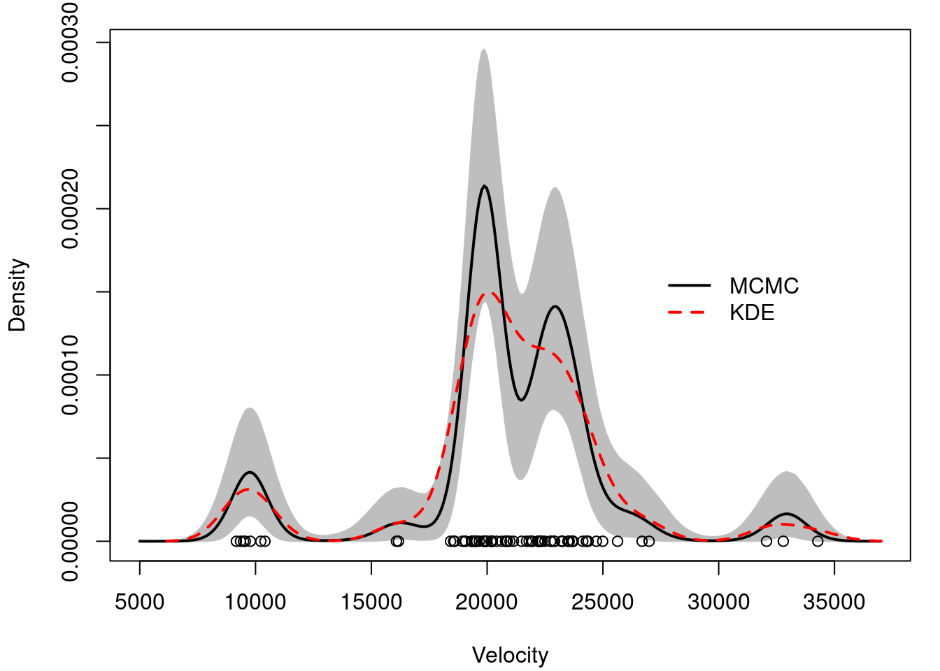
## Plot Bayesian estimate with pointwise credible bands along with kernel density estimate and frequentist point estimate
## Compute the samples of the density over a dense grid
xx  = seq(5000,37000,length=300)
density.mcmc = array(0, dim=c(rrr-burn,length(xx)))
for(s in 1:(rrr-burn)){
  for(k in 1:KK){
    density.mcmc[s,] = density.mcmc[s,] + w.out[s+burn,k]*dnorm(xx,mu.out[s+burn,k],sigma.out[s+burn])
  }
}
density.mcmc.m = apply(density.mcmc , 2, mean)

yy = density(x)
colscale = c("black", "red")
density.mcmc.lq = apply(density.mcmc, 2, quantile, 0.025)
density.mcmc.uq = apply(density.mcmc, 2, quantile, 0.975)
par(mfrow=c(1,1))
par(mar=c(4,4,1,1)+0.1)
plot(xx, density.mcmc.m, type="n",ylim=c(0,max(density.mcmc.uq)),xlab="Velocity", ylab="Density")
polygon(c(xx,rev(xx)), c(density.mcmc.lq, rev(density.mcmc.uq)), col="grey", border="grey")
lines(xx, density.mcmc.m, col=colscale[1], lwd=2)
lines(yy, col=colscale[2], lty=2, lwd=2)
points(x, rep(0,n))
legend(27000, 0.00017, c("MCMC","KDE"), col=colscale[c(1,2)], lty=c(1,2), lwd=2, bty="n")
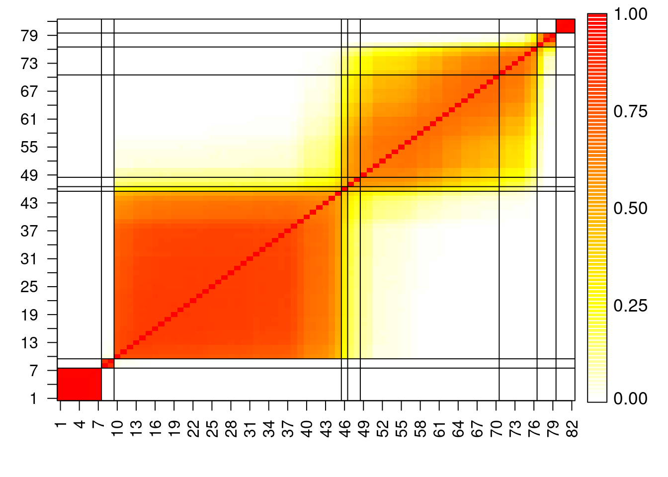
##### Finding optimal partition according to Binder's loss function
##
## Function that computes the loss at a particular configuration
Lstst = function(cch, DD, Dbar){
  z = 0
  for(i in 1:(n-1)){
    for(j in (i+1):n){
      if(cch[i]==cch[j]){
        z = z + (DD[i,j]-Dbar)
      }
    }
  }
  return(z)
}

## Initial value of the algorithm is the last iteration of the sampler
## Using as.numeric(factor()) is a cheap way to force the cluster labels
## to be sequential starting at 1
cch = as.numeric(factor(cc))

## Setup parameters for the recursive alorithm
Dbar = 0.50
optLstst.old  = -Inf
optLstst.new = Lstst(cch, DD, Dbar=Dbar)
maxiter = 50
niter   = 1
while((optLstst.old!=optLstst.new)&(niter<=maxiter)){
  for(i in 1:n){
    nq   = max(cch) + 1
    q    = rep(0, nq)
    for(s in 1:nq){
      ccht    = cch
      ccht[i] = s
      q[s] = Lstst(ccht, DD, Dbar=Dbar)
    }
    cch[i] = which.max(q)
    cch = as.numeric(factor(cch))
  }
  optLstst.old = optLstst.new
  optLstst.new = Lstst(cch, DD, Dbar=Dbar)
  niter = niter+1
}
#print(nunique(cch))

## Create another heatmap plot of the co-clustering matrix in which the
## optimal clusters are represented.
cchlo    = as.numeric(as.character(factor(cch, labels=order(unique(cch)))))
cchlotab = table(cchlo)
llc      = cumsum(cchlotab[-length(cchlotab)])
heatmapplot(DD, seq(1,n), seq(1,n,by=3), llc=llc)
#dev.print(file="galaxiesheatmap50.pdf", dev=pdf)
```