Learning Objectives
99.1 Seasonal NDLMs
This module material corresponds to a chapter 3 in Prado, Ferreira, and West (2023) titled “The frequency domain”
In practical terms though there are two sub-model used for seasonality for NDLMs
- One that uses dummy variables. Useful for assigning a repeating pattern for days of the week. These can be learned or specified,
- TODO: example for setting the weekly pattern.
- TODO: example for learning the weekly pattern.
- One that uses superposition of sinusoids. These are better smooth long range seasonal patterns and can fit them with very few parameters.
- Both come with constraint (a sum to one) so that we need to specify one less parameter than we actually require.
- The Python implementation
pyDLMhas an interesting idea for allowing us to specify both short term and long term seasonality. This idea is illustrated in the following snippet:
monthly = longSeason(period=12, stay=30, data=data, name='monthly', w=1e7)Where for example, the time unit is day, but user wants to add long term seasonality for a the 12 month resolution.
These components allow us to model processes that have structure at multi-scale in time behavior without requiring very many parameters. This is a power modeling capability that you should cultivate before you try to use NDLMs in production.
99.2 Fourier representation 🎥
In this lesson we describe how to incorporate seasonal components in a normal dynamic linear model. We start with a single Fourier component representation . This corresponds to the case where we have a single frequency, and how to incorporate that single frequency in your model for the seasonality. Then we will use the superposition principle, to incorporate multiple frequencies more specifically these take the form of a fundamental frequency and its corresponding harmonics in our NDLM.
Note: that the material is covered again in a handout reproduced below but I think at this point my notes provide more details and some insights not available in the handouts.
There are other seasonal representations clarification needed. (Petris, Petrone, and Campagnoli 2009, sec. 3.2.2) discusses seasonal factor models which Prado mentions at the very end of the video as being based on a permutation matrix together with a factor vector. This factor based representation requires one parameter per season, while the fourier representation can be more parsimonious. However I can say from my own experience that this representation can be useful if you know the daily mean for a week and which to use that as a day of the week seasonality.
For the rest of this lesson we will focus on the Fourier representation as it is both flexible and more parsimonious with regard to the parameters. E.g. If we wish to model just the fundamental frequency we can omit all the harmonics of that frequency.
We will discuss two cases :
99.2.1 Single frequency Fourier NDLM with \omega \in (0,\pi)
This gives us the following matrix representation NDLM:
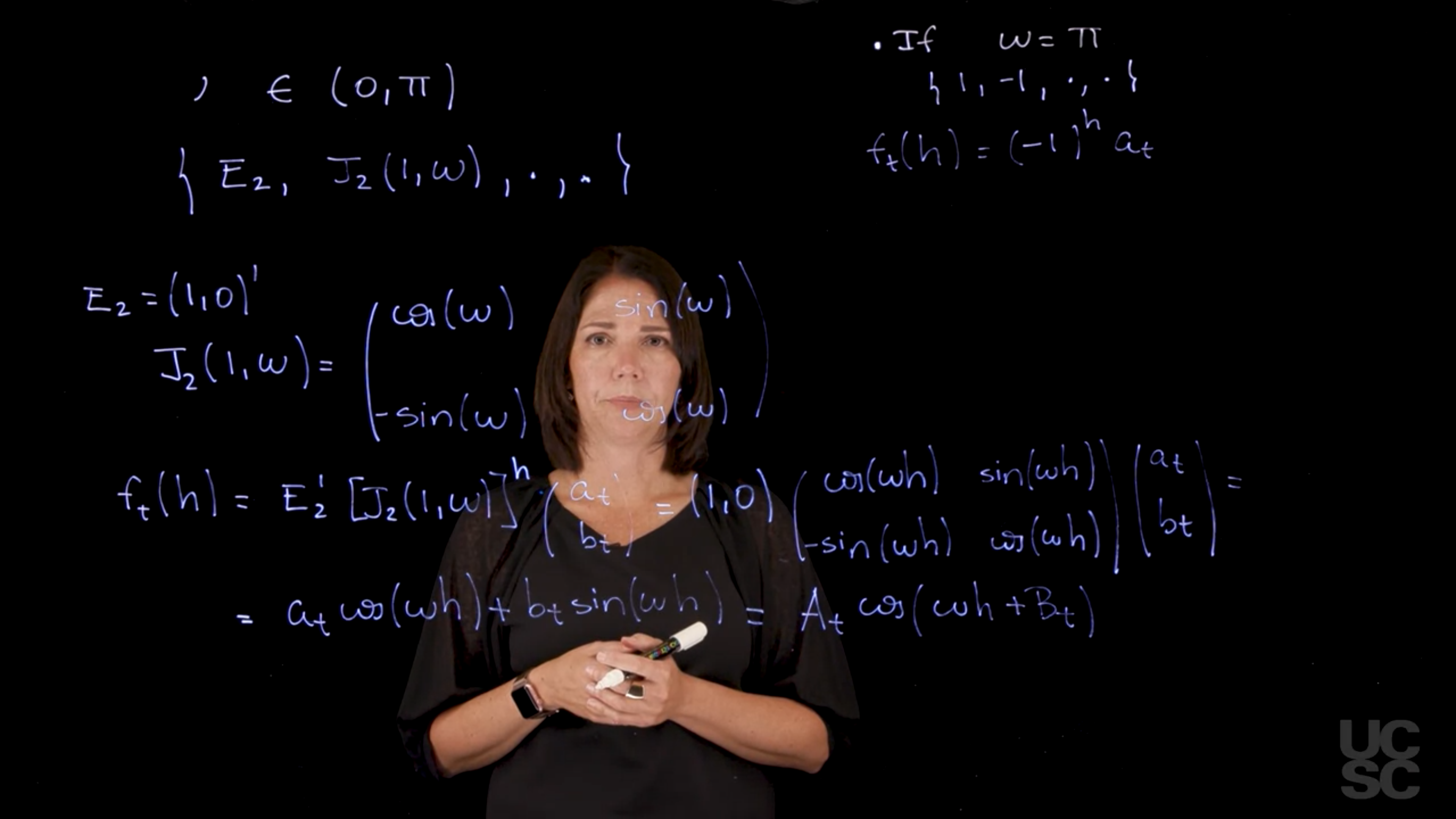
\{ \underbrace {E_2}_{F}, \underbrace {J_2(1,\omega)}_{G}, \underbrace{\cdot \vphantom{E_2}}_{V_t}, \underbrace{\cdot \vphantom{E_2}}_{W_t}\} \tag{99.1}
- where:
- E_2=(1,0)^\top
- J_2(1, \omega) = \begin{pmatrix} \cos(\omega) & \sin(\omega) \\ -\sin(\omega) & \cos(\omega) \end{pmatrix}
Since the system matrix is a 2\times 2 matrix the our state parameter vector must be a vector of dimension 2.
If we think about the forecast function, f_t(h) h-steps ahead, (you are at time t and you want to look for h steps ahead). Let’s recall: the way we work with this is F G^h a_t
\begin{aligned} f_t(h)&\stackrel{\triangle}{=}\mathbb{E}[y_{t+h} \mid \mathcal{D}_{T}] && \text{defn. of forecast fn.} \\ &= F'G^h \mathbb{E}[\theta_{t} \mid \mathcal{D}_{T}] && \text{case of const F and G} \\ &= E_2' [J_2(1, \omega)]^h \underbrace{\begin{pmatrix} a_t \\ b_t \end{pmatrix}}_{\mathbb{E}[\theta\mid \mathcal{D}_t]} && \text{subst. F and G} \\ &= (1,0) \begin{pmatrix} \cos(\omega h) & \sin(\omega h) \\ -\sin(\omega h) & \cos(\omega h) \end{pmatrix} \begin{pmatrix} a_t \\ b_t \end{pmatrix} && \text{multiplying out} \\ &= a_t \cos(\omega h) + b_t \sin(\omega h) && \text{trig identities} \\ &= \underbrace{A_t}_{\text{amplitude}} \cos(\omega h + \underbrace{B_t}_{\text{phase}}) && \blacksquare \end{aligned} \tag{99.2}
Bear in mind that this derivation is important because it will feature in the constructions used to form the multiple frequency component Fourier NDLMs.
99.2.2 Single frequency Fourier NDLM with \omega = \pi
This gives a one dimensional state vector and the following forecast function \begin{aligned} f_t(h) &= -1^h a_t \end{aligned} \tag{99.3}
99.2.3 Multiple frequency component Fourier NDLM for odd p
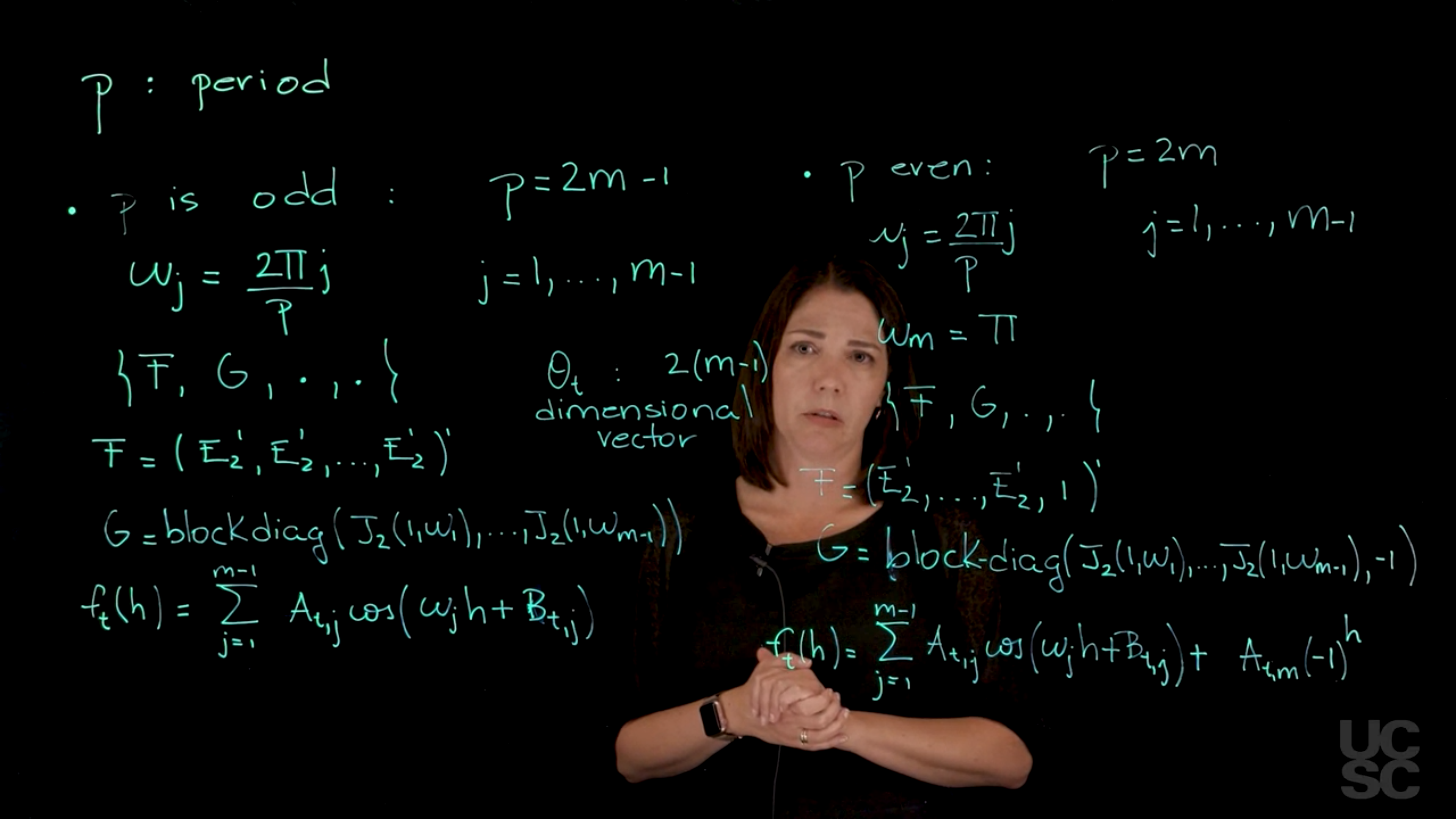
Next we look at multiple frequencies, again we have two cases and we start with the case where the period p is odd. Since p is odd we can write it a p=2m-1 for some integer m.
- How many frequencies will we be able to incorporate in this model?
Since
\omega_j = \frac{2\pi j}{p}, \qquad j = 1, \ldots, m-1 \tag{99.4}
Now we can use the superposition principle thinking we have a component DLM representation for each of these frequencies. They are all going to be between 0 and \pi.
For each frequency we get a two-dimensional DLM representation in terms of the state vector. We use the superposition principle to concatenate them all and get a model that incorporates all these frequencies.
- How are the frequencies related?
There is one frequency associated with the fundamental period and all its harmonics.
Now to the model our F and my G are both going to be constant over time so we can drop the t subscript. Giving us:
\{ F,G, \cdot, \cdot \} \tag{99.5}
For the F we need to concatenate as many E_2^\top as we have frequencies \omega I’m going to have E_2 transpose and we have m-1 such components.
F = (E_2^\top,E_2^\top,...,E_2^\top,)^\top \tag{99.6}
Since each E_2^\top has dimension 2 we get a parameter vector \theta_t with dimension of 2 times m-1.
Next we consider the System Evolution matrix G. We construct it by concatenating the J_2(1, \omega_j) matrices for each frequency j in a block diagonal form which gives us
G = \text{blockdiag}[J_2(1, \omega_1), \ldots, J_2(1, \omega_{m-1})] \tag{99.7}
which is compatible with the \theta_t we use.
- What is the form of the forecast function in this case ?
Again, using the superposition principle, the forecast function is going to be just the sum of m minus 1 components, where each of those components is going to have an individual forecast function that has that cosine wave representation that we discussed before. This gives us the h step forecast function at time t as follows: f_t(h) = \sum_{j=1}^{m-1} A_{t,j} \cos(\omega_j h + B_{t,j}) \tag{99.8}
- where:
- j is the index for
- \omega_j the frequency
- A_{t,j} the amplitude and
- B_{t,j} the phase
So once again we have an amplitude and phase for each of the components and so it depends on time t but does not depend on h.
The h appears in a product with the frequency.
99.2.4 Multiple frequency component Fourier NDLM for even p
In the case of even p the situation is slightly different.
But again, it’s the same in terms of using the superposition principle. In this case, we can write down P as 2 times m because it’s an even number.
For even p we write p=2m for some integer m.
We write these frequencies \omega_j as a function of the fundamental period. This time the index runs from 1 up to m-1. \omega_j = \frac{2\pi j}{p}, \qquad j = 1, \ldots, m-1 \tag{99.9}
For the last frequency, when j=m, this simplifies to be the Nyquist frequency. In this case, we get
\omega_m= \pi \tag{99.10}
the model is
\{ F,G, \cdot, \cdot \} \tag{99.11}
In this particular case, when I concatenate everything, we get F and a G that look like this:
F = (E_2^\top, E_2^\top, \ldots, E_2^\top,1)^\top \tag{99.12}
where the last component is just a 1, which corresponds to the Nyquist frequency.
Then G is going to be the block diagonal.
G = \text{blockdiag}[J_2(1, \omega_1), \ldots, J_2(1, \omega_{m-1})] \tag{99.13}
For the last frequency I have that minus 1. This determines the dimension of the state vector, in this case I’m going to have 2 times m minus 1 plus 1.
The forecast function
For the My f function, my forecast function, is again a function of the number of steps ahead. We get the same structure we had before for the m- 1 components. Then we have to add one more component that corresponds to the frequency \pi.
f_t(h) = \sum_{j=1}^{m-1} A_{t,j} \cos(\omega_j h + \gamma_{t,j}) + (-1)^h A_{t,m} \tag{99.14}
where A_{t,m} is the amplitude for the Nyquist frequency and it takes the sign based on the power of h.
Once again we employ the superposition principle to go from component representation to the full Fourier representation.
In practice, once we set the period, we can use a model that has the fundamental period and all the harmonics related to that fundamental period.
However, we may also choose to discard some of those harmonics and use a subset of them. This is the flexibility that the Fourier representation allows.
99.2.5 Seasonal Factor representation
There are other representations that are also used in practice. One of them is the seasonal factors representation. In that case, you’re going to have a model in which the state vector has dimension p for a given period.
It uses a G matrix that is a permutation matrix. There is a correspondence between this parameterization using the Fourier representation and the Factor representation
If you want to use that parameterization, the way to interpret the components of this state vector, since you have P of those, is going to be a representation in terms of factors.
For example, if you think about monthly data, you will have the say January factor, February factor, March factor, and so on.
You could think about those effects and do a correspondence with this particular model. We will always work in this class with the fourier representations because it’s more flexible.
But again, we can go back and forth between one and the other.
I will now describe how to incorporate seasonal components in a normal dynamic linear model. What we will do is we will first talk about the so-called single Fourier component representation. Just in case you have a single frequency and how to incorporate that single frequency in your model for the seasonality. Then using the superposition principle, you can incorporate several frequencies or a single frequency and the corresponding harmonics in your model. Let’s begin with that. There are other seasonal representations as well. I will just focus on the Fourier representation because it allows you to have a lot of flexibility without having a lot of parameters, in case you want to consider, for example, a fundamental frequency but you don’t want all the harmonics of that frequency. The Fourier representation, if you happen to have a single frequency. We will discuss two cases. The case in which the frequency is between zero and Pi, so this is your Omega frequency, any frequency between zero and Pi. Then we will describe the case in which the frequency is exactly Pi, so the component representation is different. In the case of any frequency in this range, you’re going to have dynamic linear model that has this structure. You will have the F vector is going to be a two-dimensional vector. The first component is one, the second component is zero. This is the usual 1,0 here. Then you’re going to have this G, which I will describe in a minute, then you have your corresponding v_t and W_t, wherever you want to put in here. In the case of the G matrix, that’s the matrix for your model, is going to have this form. It’s a two-by-two matrix so your state parameter vector is also a state parameter vector of dimension 2. You’re going to have the cosine of the frequency here, the sine of the frequency. That’s your G matrix. If you think about the forecast function, h steps ahead, so you are at time t and you want to look for h steps ahead. If you remember, the way we work with this is going to be your E_2 transpose, then you have to take this G matrix, which is just this J_2^1 Omega, to the power of h, and then you have a vector, I’m going to call a_t and b_t, which is just going to be this vector value of your Theta t vector given the information up to the time t. It’s going to have two components, I’m just going to generically call them a_t and b_t. When you take this to the power of h using just trigonometric results, you’re going to get that J_2^1,Omega to the power of h is just going to give you cosine of Omega h sine of Omega h minus sine of Omega h cosine of Omega h. When you look at this expression, you get something that looks like this, and then you have, again, times these a_t, b_t. You’re going to have the cosine and sine only multiplied by this. In the end, you’re going to have something that looks like this. You have this sinusoidal form with the period Omega in your forecast function. You can also write this down in terms of an amplitude that I’m going to call A_t and then a phase that is B_t. Here again, you have your periodicity that appears in this cosine wave. This is again for the case in which you have a single frequency and the frequencies in this range. There was a second case that I mentioned, and that case is the case in which the Omega is exactly Pi. In this case, your Fourier representation is going to be your model that has a state vector that is just one dimensional. In the case where Omega is between zero and Pi, you have a two-dimensional state, vector here you’re going to have a one-dimensional state vector. This is going to be your F and your G. Then you have again whatever you want to put here as your v_t and W_t. This gives me, if I think about the forecast function, h steps ahead is just going to be something that has the form minus 1^h times a_t. Now I have a single component here, is uni-dimensional. This is going to have an oscillatory behavior between a_t and minus a_t if I were to look h steps ahead forward when I’m at time t. These two forms give me the single component Fourier representation and using the superposition principle, we will see that we can combine a single frequency and the corresponding harmonics or several different frequencies just using the superposition principle in the normal dynamic linear model. You can also incorporate more than one component in a full Fourier representation. Usually the way this works is you have a fundamental period, let’s say p. For example, if you are recording monthly data, p could be 12 and then you are going to incorporate in the model the fundamental frequency, and then all the harmonics that go with that fundamental frequency related to the period p. Here p, is the period and in this case, we are going to discuss essentially two different situations. One is when p is an odd number, the other one is when p is an even number. Let’s begin with the case of p is odd and in this particular scenario, we can write down p as 2 times m minus 1 for some value of m. This gives me a period that is odd. How many frequencies I’m going to incorporate in this model? I’m going to be able to write down Omega j as 2 Pi times j over p, which is the fundamental period. j here goes from one all the way to m minus 1. Now we can use the superposition principle thinking we have a component DLM representation for each of these frequencies. They are all going to be between 0 and Pi. For each of them I’m going to have that two-dimensional DLM representation in terms of the state vector and then I can use the superposition principle to concatenate them all and get a model that has all these frequencies, the one related to the fundamental period and all the harmonics for that. Again, if I think about what is my F and my G here, I’m not writing down the t because both F and G are going to be constant over time. So my F is going to be again, I concatenate as many E_2 as I have frequencies in here. I’m going to have E_2 transpose and so on and I’m going to have m minus one of those. Times 2 gives me the dimension of Theta t. The vector here is 2 times m minus 1 dimensional vector. My G is going to have that block diagonal structure where we are going to just have all those J_2 1 Omega 1, all the way down to the last harmonic. Each of these blocks is a two-by-two matrix and I’m going to put them together in a block diagonal form. This gives me the representation when the period is odd, what is the structure of the forecast function? Again, using the superposition principle, the forecast function is going to be just the sum of m minus 1 components, where each of those components is going to have an individual forecast function that has that cosine wave representation that we discussed before. Again, if I think about the forecast function at time t h steps ahead, I will be able to write it down like this. This should be a B. B_t,j. Again here, I have an amplitude for each of the components and a phase for each of the components so it depends on time but does not depend on h. The h enters here, and this is my forecast function. In the case of P even the situation is slightly different. But again, it’s the same in terms of using the superposition principle. In this case, we can write down P as 2 times m because it’s an even number. Now I can write down these Omega j’s as a function of the fundamental period. Again, this goes from 1 up to m minus 1. But there is a last frequency here. When j is equal to m, this simplifies to be the Nyquist frequency. In this case, I have my Omega is equal to Pi. In this particular case, when I concatenate everything, I’m going to have again an F and a G that look like this. Once again, I concatenate all of these up to the component m minus 1. Then I have this 1 for the last frequency. Then my G is going to be the block diagonal. For the last frequency I have that minus 1. This determines the dimension of the state vector, in this case I’m going to have 2 times m minus 1 plus 1. My f function, my forecast function, is again a function of the number of steps ahead. I’m going to have the same structure I had before for the m minus 1 components. Then I have to add one more component that corresponds to the frequency Pi. This one appears with the power of h. As you can see, I’m using once again the superposition principle to go from component representation to the full Fourier representation. In practice, once we set the period, we can use a model that has the fundamental period and all the harmonics related to that fundamental period. We could also use, discard some of those harmonics and use a subset of them. This is one of the things that the Fourier representation allows. It allows you to be flexible in terms of how many components you want to add in this model. There are other representations that are also used in practice. One of them is the seasonal factors representation. In that case, you’re going to have a model in which the state vector has dimension p for a given period. It uses a G matrix that is a permutation matrix. There is a correspondence between this parameterization using the Fourier representation and that other parameterization. If you want to use that parameterization, the way to interpret the components of this state vector, since you have P of those, is going to be a representation in terms of factors. For example, if you think about monthly data, you will have the say January factor, February factor, March factor, and so on. You could think about those effects and do a correspondence with this particular model. We will always work in this class with these representations because it’s more flexible. But again, you can go back and forth between one and the other.
99.3 Fourier Representation: Example 1 🗒️
The following example is from a handout
99.3.1 Seasonal Models
Example: Full Fourier Model with p=5
In this case the Fourier frequencies are
- \omega_1 = 2\pi/5 and \omega_2 = 4\pi/5 and so on
- p = 2 × 3 − 1. Then, m = 3 and
- \theta_t = (\theta_{t,1}, \ldots , \theta_{t,4})\top,
- F = (1, 0, 1, 0)^\top,
- G is given by:
G = \begin{pmatrix} \cos(2\pi/5) & \sin(2\pi/5) & 0 & 0 \\ \cos(2\pi/5) & \sin(2\pi/5) & 0 & 0 \\ 0 & 0 & \cos(4\pi/5) & \sin(4\pi/5) \\ 0 & 0 & \cos(4\pi/5) & \sin(4\pi/5) \\ \end{pmatrix}
and the forecast function is:
f_t(h) = A_{t,1} \cos(2\pi h/5 + \gamma_t) + A_{t,2} \cos(4\pi h /5 + \gamma_{t,2}) \qquad \tag{99.15}
99.4 Building NDLMs with Multiple Components: Examples 🎥
In this example, we are going to have two components:
- a linear trend plus
- a seasonal component where the fundamental period is four.
The way we construct such a model, is via the superposition principle
- “what structure do we need, to get a linear trend in the forecast function ?”
The linear trend is a linear function on the number of steps ahead.
Whenever we want that structure, we will use a DLM that we call a polynomial model of order 2.
Professor Prado isn’t clear enough here so let me try to clarify:
We have options here for the linear trend. Polynomial models are a class of models that allow us to incorporate linear trends. They are smooth, and linear and we typically only polynomials of order 1 and 2. Order 1 correspond to having a mean and order 2 corresponds to having a mean and a gradient in the trend.
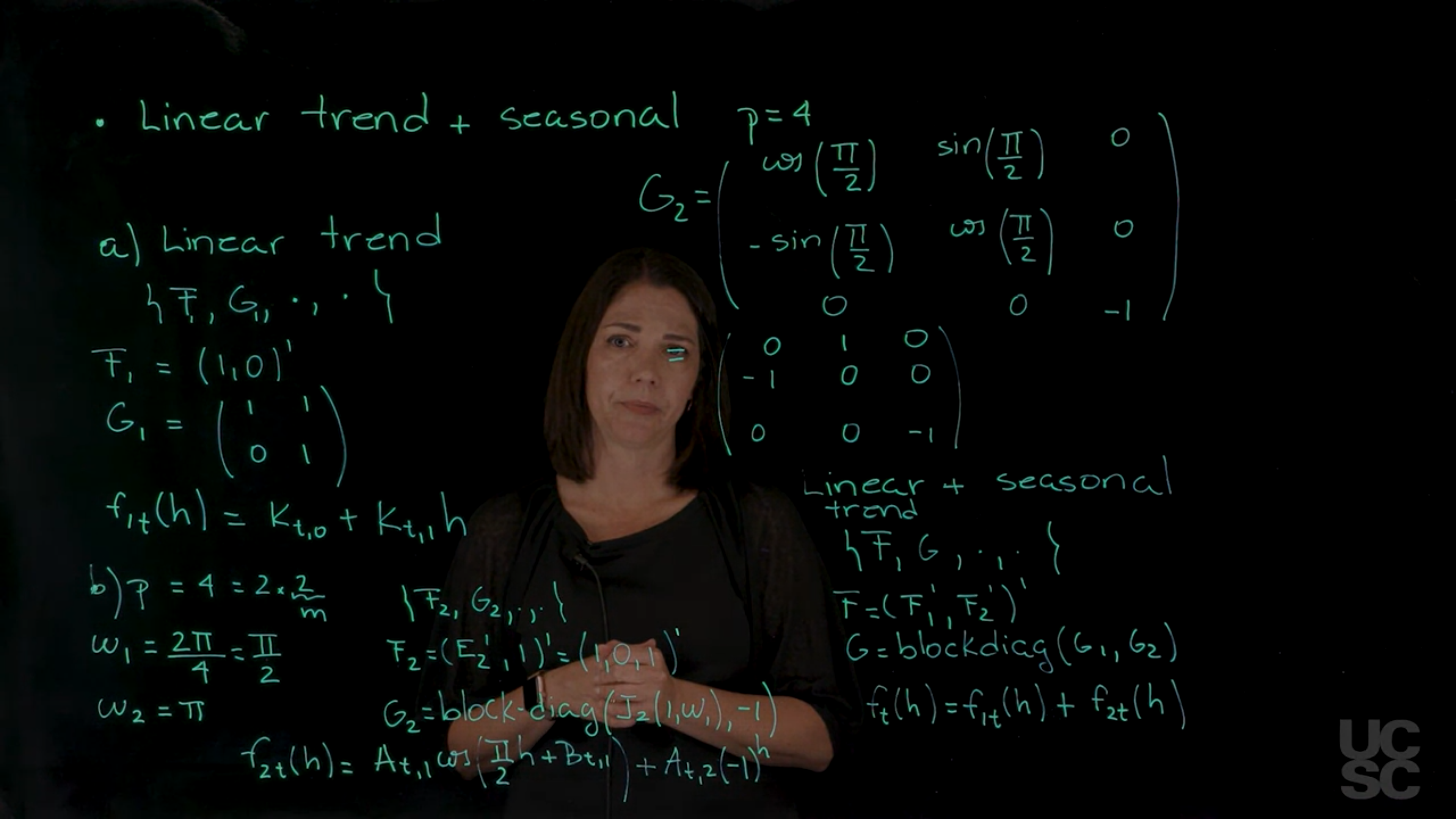
So let’s discuss first the linear component it looks like \{F_1, G_1, \cdot, \cdot\} where we index F, G using one the to denote that this is the first component in the model.
F_1 = \begin{pmatrix} 1 & 0 \end{pmatrix}^\top
G_1 = \begin{pmatrix} 1 & 1 \\ 0 & 1 \end{pmatrix}
Next we can write down the forecast function, let’s call it f_{1,t}(h) in terms of the number of steps ahead is just a linear function on h, is a linear polynomial order 1.
f_{1,t}(h) = K_{t,0} + K_{t,1} h
This is the structure of the first component.
Next we have to think about the seasonal component with period of four.
If we are going to incorporate all the harmonics, we need to check is this an even period or a not period?
In this example, p=4=2*m \implies m=2 so it is an even period.
We are going to have one frequency, the first one, \omega_1, is related to the fundamental period of 4, so it is is {2 \pi} \over {4}, which I can simplify and write down this as \pi \over 2.
The last one is going to correspond to the Nyquist.
\{F_2,G_2,\cdot,\cdot\}
with
F_2=\begin{pmatrix} 1 & 0 & 1 \end{pmatrix}^\top
\begin{aligned} G_2&= \text{blockdiag}[J_2(1, \omega_1), -1] \\ &= \begin{pmatrix} \cos(\frac{\pi}{2}) & \sin(\frac{\pi}{2}) & 0 \\ -\sin(\frac{\pi}{2}) & \cos(\frac{\pi}{2}) & 0 \\ 0 & 0 & -1 \end{pmatrix} \\ &= \begin{pmatrix} 0 & 1 & 0 \\ -1 & 0 & 0 \\ 0 & 0 & -1 \end{pmatrix} \end{aligned}
Now we can combine the the components into our desired model
\{F,G,\cdot\cdot\}
F = (F_1^\top,F_2^\top)
G = (G_1,G_2)
What is this models dimensions?
Since the first component G_2 is going to have dimension 2 and the second is going to have dimension 3 the model is going to be five-dimensional.
We could add regression components, autoregressive components etc. All of these models are using, again, the superposition principle and the fact that we’re working with a linear and Gaussian structure in terms of doing the posterior inference later.
In this second example, we are going to have two components; a linear trend plus a seasonal component where the fundamental period is four. The way to build this model, again, is using the superposition principle. We first think about what is the structure we need to have a linear trend in the FORECAST function. The linear trend is a linear function on the number of steps ahead. Whenever you have that structured, you are going to have a DLM that is the so-called polynomial model of order 2, so let’s discuss first the linear. Let’s say the linear trend part, and in this case, we have an F and a G, I’m going to call them 1, F_1 and G_1 to denote that this is the first component in the model. F_1 is just going to be 1, 0 transpose, and the G_1 is that upper triangular matrix, it’s a 2 by 2 matrix that has 1, 1 in the first row, 0, 1 in the second row, so this gives me a linear trend. My forecast function, let’s call it f_1t in terms of the number of steps ahead is just a linear function on h, is a linear polynomial order 1. Let’s say it’s a constant of K but depends on t0 plus K_t1 h. This is the structure of the first component. Then I have to think about the seasonal component with period of four. If we are going to incorporate all the harmonics, we have to think again, is this an even period or a not period? In this example, this is an even period. I can write p, which is 4, as 2 times 2, so this gives me that m. I’m going to have one frequency, the first one, Omega 1, is related to the fundamental period of 4, so is 2 Pi over 4, which I can simplify and write down this as Pi over 2. This is the first frequency. The last one is going to correspond to the Nyquist. We could obtain that doing 4Pi over 4, which is just Pi. As you remember, this component is going to require a two-dimensional DLM component model, this one is going to require a one-dimensional DLM component model in terms of the dimension here is the dimension of the state vectors. When we build this concatenating these components, we are going to have, again, let’s call it F_2 and G_2 for this particular component. I had called this here a, let’s call this b. My F_2 has that E_2 transpose and a 1, which gives me just 1, 0, 1. My G matrix is going to be a 3 by 3 matrix. The first component is the component associated to that fundamental period. It’s a block diagonal again, and I’m going to have that J_2, 1 Omega 1, and then I have my minus 1 here. What this means is if I write this down as a matrix, let me write it here, G_2 is going to be cosine of that Pi halves, and then I have zeros here, I have my minus 1 here, 0, and 0. I can further simplify these to have this structure. The cosine of Pi halves is 0, the sine is 1, so I can write this down as 0, 1, 0, minus 1, 0, 0, and 0, 0 minus 1. Now if I want to go back to just having a model that has both components, I use the superposition principle again and combine this component with this component. The linear plus seasonal is a model that is going to have the representation F, G, with F is going to be just concatenate F_1 and F_2. G now has that block diagonal form again. If I look at what I have, I have this block that is a 2 by 2, this block that is a 3 by 3. Therefore my model is going to be a five-dimensional model in terms of the state parameter vector, so this G is a 5 by 5, and this one is also a five-dimensional vector. Finally, if I think about the forecast function in this case, if I call here the forecast function f_2t for the component that is seasonal, I’m going to have my A_t1 cosine of Pi halves h plus B_t1, and then I have my A_t2 minus 1^h. My forecast function for the final model is going to be just the sum of these two components. You can see how I can now put together all these blocks, so I have a block that is seasonal and a block that is a linear polynomial model, and I can put them together in a single model just to create a more flexible structure. You could add regression components, you could add autoregressive components and put together as many components as you need for the forecast function to have the form that you expect it to have. All of these models are using, again, the superposition principle and the fact that we’re working with a linear and Gaussian structure in terms of doing the posterior inference later.
99.5 Summary: DLM Fourier representation 🗒️
99.5.1 Seasonal Models: Fourier Representation
For any frequency \omega \in (0, \pi), a model of the form \{E_2, J_2(1, \omega), \cdot, \cdot\} with a 2-dimensional state vector \theta_t = (\theta_{t,1}, \theta_{t,2})' and
J_2(1, \omega) = \begin{pmatrix} \cos(\omega) & \sin(\omega) \\ -\sin(\omega) & \cos(\omega) \end{pmatrix},
has a forecast function:
\begin{aligned} f_t(h) &= (1, 0) J_2^h(1, \omega) (a_t, b_t) \\ &= a_t \cos(\omega h) + b_t \sin(\omega h) \\ &= A_t \cos(\omega h + B_t). \end{aligned}
For \omega = \pi, the NDLM is \{1, -1, \cdot, \cdot\} and has a forecast function of the form
f_t(h) = (-1)^h m_t
These are component Fourier models. Now, for a given period p, we can build a model that contains components for the fundamental period and all the harmonics of such a period using the superposition principle as follows:
99.5.2 Case: p = 2m - 1 (odd)
Let \omega_j = 2\pi j / p for j = 1 : (m - 1), F a (p - 1)-dimensional vector, or equivalently, a 2(m - 1)-dimensional vector, and G a (p - 1) \times (p - 1) matrix with F = (E_2', E_2', \dots, E_2')',
G = \text{blockdiag}[J_2(1, \omega_1), \dots, J_2(1, \omega_{m-1})].
99.5.3 Case: p = 2m (even)
In this case, F is again a (p - 1)-dimensional vector (or equivalently a (2m - 1)-dimensional vector), and G is a (p - 1) \times (p - 1) matrix such that F = (E_2', \dots, E_2', 1)' and
G = \text{blockdiag}[J_2(1, \omega_1), \dots, J_2(1, \omega_{m-1}), -1].
In both cases, the forecast function has the general form:
f_t(h) = \sum_{j=1}^{m-1} A_{t,j} \cos(\omega_j h + \gamma_{t,j}) + (-1)^h A_{t,m},
with A_{t,m} = 0 if p is odd.
99.6 Examples
99.6.1 Fourier Representation, p = 12:
In this case, p = 2 \times 6 so \theta_t is an 11-dimensional state vector
F = (1, 0, 1, 0, 1, 0, 1, 0, 1, 0, 1)',
the Fourier frequencies are \omega_1 = 2\pi/12, \omega_2 = 4\pi/12 = 2\pi/6, \omega_3 = 6\pi/12 = 2\pi/4, \omega_4 = 8\pi/12 = 2\pi/3, \omega_5 = 10\pi/12 = 5\pi/6, and \omega_6 = 12\pi/12 = \pi (the Nyquist frequency).
G = \text{blockdiag}(J_2(1, \omega_1), \dots, J_2(1, \omega_5), 1)
and the forecast function is given by:
f_t(h) = \sum_{j=1}^{5} A_{t,j} \cos(2\pi j / 12 + \gamma_{t,j}) + (-1)^h A_{t,6}.
99.6.2 Linear Trend + Seasonal Component with p = 4
We can use the superposition principle to build more sophisticated models. For instance, assume that we want a model with the following 2 components:
- Linear trend: \{F_1, G_1, \cdot, \cdot\} with F_1 = (1, 0)',
G_1 = J_2(1) = \begin{pmatrix} 1 & 1 \\ 0 & 1 \end{pmatrix}.
- Full seasonal model with p = 4: \{F_2, G_2, \cdot, \cdot\}, p = 2 \times 2 so m = 2 and \omega = 2\pi / 4 = \pi / 2,
F_2 = (1, 0, 1)',
and
G_2 = \begin{pmatrix} \cos(\pi / 2) & \sin(\pi / 2) & 0 \\ -\sin(\pi / 2) & \cos(\pi / 2) & 0 \\ 0 & 0 & -1 \end{pmatrix} = \begin{pmatrix} 0 & 1 & 0 \\ -1 & 0 & 0 \\ 0 & 0 & -1 \end{pmatrix}.
The resulting DLM is a 5-dimensional model \{F, G, \cdot, \cdot\} with
F = (1, 0, 1, 0, 1)',
and
G = \begin{pmatrix} 1 & 1 & 0 & 0 & 0 \\ 0 & 1 & 0 & 0 & 0 \\ 0 & 0 & 0 & 1 & 0 \\ 0 & 0 & -1 & 0 & 0 \\ 0 & 0 & 0 & 0 & -1 \end{pmatrix}.
The forecast function is:
f_t(h) = (k_{t,1} + k_{t,2} h) + k_{t,3} \cos(\pi h / 2) + k_{t,4} \sin(\pi h / 2) + k_{t,5} (-1)^h.