---
date: 2024-10-23
title: "Homework - MLE and Bayesian inference in the AR(1)"
subtitle: Time Series Analysis
description: "This lesson we will define the AR(1) process, Stationarity, ACF, PACF, differencing, smoothing"
categories:
- Bayesian Statistics
keywords:
- time series
- stationarity
- strong stationarity
- weak stationarity
- lag
- autocorrelation function (ACF)
- partial autocorrelation function (PACF)
- smoothing
- trend
- seasonality
- differencing operator
- back shift operator
- moving average
---
\index{dataset,EEG}
This peer-reviewed activity is highly recommended. It does not figure into your grade for this course, but it does provide you with the opportunity to apply what you've learned in R and prepare you for your data analysis project in week 5.
1) Consider the R code in @lst-ar-1-mle-unmodified
```{r}
#| label: lst-ar-1-mle-unmodified
#| lst-label: lst-ar-1-mle-unmodified
#| lst-cap: "MLE for the AR(1)"
####################################################
#####             MLE for AR(1)               #####
####################################################
phi=0.9 # ar coefficient
v=1
sd=sqrt(v) # innovation standard deviation
T=500 # number of time points
yt=arima.sim(n = T, model = list(ar = phi), sd = sd)

## Case 1: Conditional likelihood
y=as.matrix(yt[2:T]) # response
X=as.matrix(yt[1:(T-1)]) # design matrix
phi_MLE=as.numeric((t(X)%*%y)/sum(X^2)) # MLE for phi
s2=sum((y - phi_MLE*X)^2)/(length(y) - 1) # Unbiased estimate for v
v_MLE=s2*(length(y)-1)/(length(y)) # MLE for v

cat("\n MLE of conditional likelihood for phi: ", phi_MLE, "\n",
    "MLE for the variance v: ", v_MLE, "\n",
    "Estimate s2 for the variance v: ", s2, "\n")
```
```{r}
#| label: fig-ar-1-mle-plot-1
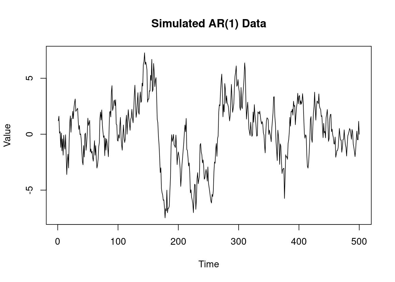
#| fig-cap: "Simulated AR(1) data"
plot(yt,
     type = "l", main = "Simulated AR(1) Data",
     xlab = "Time", ylab = "Value")
```
```{r}
#| label: lst-ar-1-posterior-inference-unmodified
#| lst-label: lst-ar-1-posterior-inference-unmodified
#| lst-cap: "AR(1) Bayesian inference, conditional likelihood"
#######################################################
###### Posterior inference, AR(1) ###
###### Conditional Likelihood + Reference Prior ###
###### Direct sampling ###
#######################################################
n_sample=3000 # posterior sample size
## step 1: sample posterior distribution of v from inverse gamma distribution
v_sample=1/rgamma(n_sample, (T-2)/2, sum((yt[2:T] - phi_MLE*yt[1:(T-1)])^2)/2)
## step 2: sample posterior distribution of phi from normal distribution
phi_sample=rep(0,n_sample)
for (i in 1:n_sample){
phi_sample[i]=rnorm(1, mean = phi_MLE, sd=sqrt(v_sample[i]/sum(yt[1:(T-1)]^2)))}
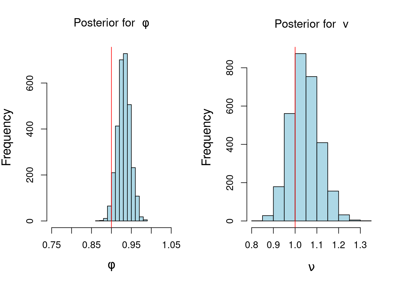
## plot histogram of posterior samples of phi and v
par(mfrow = c(1, 2), cex.lab = 1.3)
hist(phi_sample, xlab = bquote(phi),
main = bquote("Posterior for "~phi),xlim=c(0.75,1.05), col='lightblue')
abline(v = phi, col = 'red')
hist(v_sample, xlab = bquote(nu), col='lightblue', main = bquote("Posterior for "~v))
abline(v = sd, col = 'red')
```
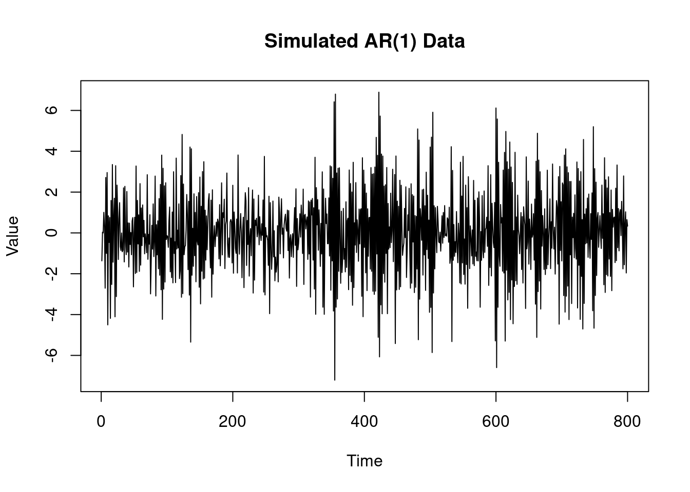
Modify the code above to sample 800 observations from an AR(1) with AR coefficient
$\phi=−0.8$ and variance $v=2$. Plot your simulated data. Obtain the MLE for
$\phi$ based on the conditional likelihood and the unbiased estimate $s^2$ for the variance $v$.
```{r}
#| label: lbl-ar-1-mle-solution
#| lst-label: lbl-ar-1-mle-unmodified
####################################################
#####             MLE for AR(1)               #####
####################################################

rm(list=ls()) # clear workspace

phi=-0.8    # ar coefficient (modified  )
v=2        # variance (modified)
sd=sqrt(v) # innovation standard deviation
T=800      # number of time points (modified)
yt=arima.sim(n = T, model = list(ar = phi), sd = sd)

## Case 1: Conditional likelihood
y=as.matrix(yt[2:T]) # response
X=as.matrix(yt[1:(T-1)]) # design matrix
phi_MLE=as.numeric((t(X)%*%y)/sum(X^2)) # MLE for phi
s2=sum((y - phi_MLE*X)^2)/(length(y) - 1) # Unbiased estimate for v
v_MLE=s2*(length(y)-1)/(length(y)) # MLE for v

cat("\n MLE of conditional likelihood for phi: ", phi_MLE, "\n",
    "MLE for the variance v: ", v_MLE, "\n",
    "Estimate s2 for the variance v: ", s2, "\n")
```
```{r}
#| label: fig-ar-1-mle-plot-2
#| fig-cap: "Simulated AR(1) data"
plot(yt,
     type = "l", main = "Simulated AR(1) Data",
     xlab = "Time", ylab = "Value")
```
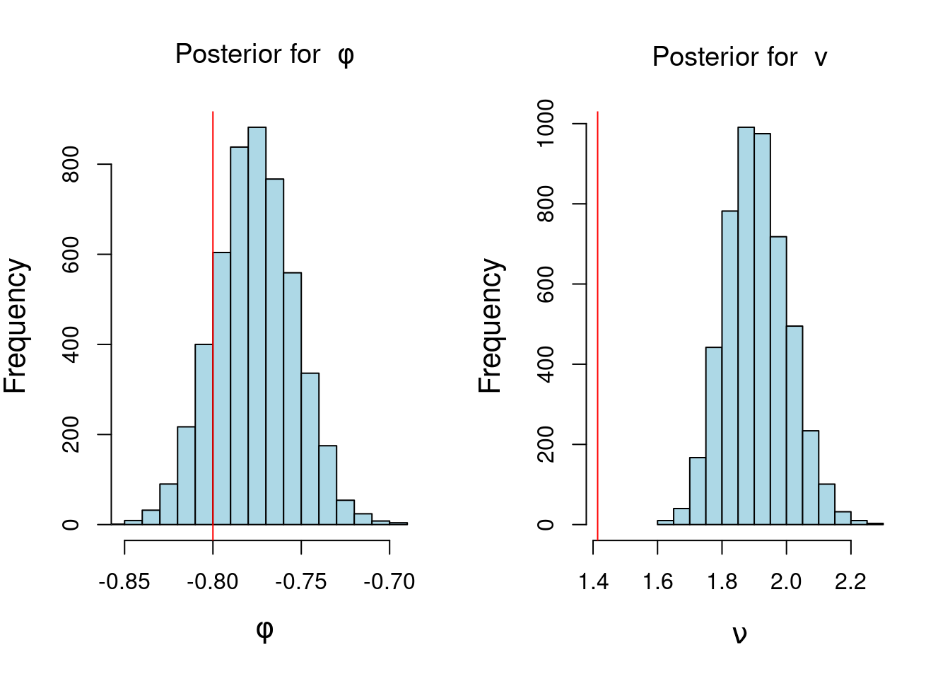
2) Consider the R code in @lst-ar-1-posterior-inference-unmodified . Using your simulated data from part 1 modify the code above to summarize your posterior inference for
$\phi$ and $\nu$ based on 5000 samples from the joint posterior distribution of $\phi$ and $\nu$.
```{r}
#| label: lst-ar-1-posterior-inference-solution
#| lst-label: lst-ar-1-posterior-inference-solution
#| lst-cap: "AR(1) Bayesian inference, conditional likelihood"
#######################################################
######     Posterior inference, AR(1)               ###
######     Conditional Likelihood + Reference Prior ###
######     Direct sampling                          ###
#######################################################

n_sample=5000   # posterior sample size (modified)

## step 1: sample posterior distribution of v from inverse gamma distribution
v_sample=1/rgamma(n_sample, (T-2)/2, sum((yt[2:T] - phi_MLE*yt[1:(T-1)])^2)/2)

## step 2: sample posterior distribution of phi from normal distribution
phi_sample=rep(0,n_sample)
for (i in 1:n_sample){
phi_sample[i]=rnorm(1, mean = phi_MLE, sd=sqrt(v_sample[i]/sum(yt[1:(T-1)]^2)))}

## plot histogram of posterior samples of phi and v
par(mfrow = c(1, 2), cex.lab = 1.3)
hist(phi_sample,
     xlab = bquote(phi),
     main = bquote("Posterior for "~phi),
     xlim=c(min(phi_sample),max(phi_sample)),
     col='lightblue')
abline(v = phi, col = 'red')
hist(v_sample,
     xlab = bquote(nu),
     col='lightblue',
     xlim=c(min(v_sample,sd),max(v_sample)),
     main = bquote("Posterior for "~v))
abline(v = sd, col = 'red')
```
note that the red line in the histogram of $\phi$ is the true value of $\phi$ and the red line in the histogram of $\nu$ is the true value of $v$. However
::::: {.content-visible unless-profile="HC"}
::: {.callout-caution}
Section omitted to comply with the Honor Code
:::
:::::
::::: {.content-hidden unless-profile="HC"}
:::::