---
title: "Hierarchical modeling - M4L11"
subtitle: "Bayesian Statistics: Techniques and Models"
description: "An overview of hierarchical modeling in the context of Bayesian statistics."
categories:
- Monte Carlo Estimation
keywords:
- hierarchical modeling
- Bayesian statistics
- R programming
- statistical modeling
- multilevel models
- group-level effects
- random effects
- hierarchical priors
- Bayesian inference
---
## Introduction to Hierarchical Modeling
{#fig-s10-hmodeling .column-margin width="53mm" group="slides"}
::: {.callout-tip}
## What about correlated data?
While the section shows the presence of correlation within groups, I wonder if we really need the iid assumptions below, particularly as we are told in [@McElreath2020Rethinking] that hierarchical models can handle correlated **data**.
:::
Throughout the last few lessons, we have assumed that all the observations were independent. But more often than not, this is too strong an assumption to make about our data. There is often a natural grouping to our data points, which leads us to believe that some observation pairs should be more similar to each other than to others.
Let's look at an example. In the previous course, we talked about using a Poisson model to count chocolate chips in cookies.
\index{chocolate chip cookies}
Let's suppose that you own a company that produces chocolate chip cookies.
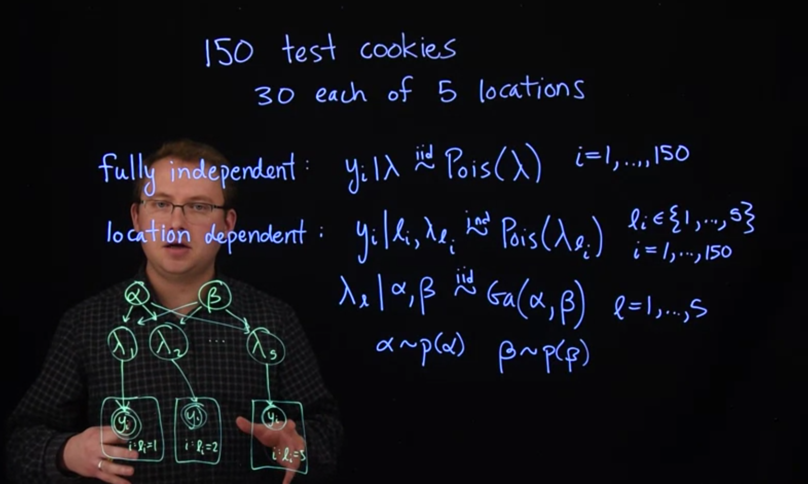
In an experiment, you're going to produce 150 test cookies.
Let's say you'll do 30 from your location and then 30 from four other factory locations.
So let's write this as 30 from each of 5 locations.
We're going to assume that all the locations use the same recipe when they make their chocolate chip cookies.
[Should we expect a cookie from your location, batch one, to be more similar to another cookie from that batch than to a cookie from another location's batch?]{.column-margin}
I'd say probably.
There's a natural grouping to the cookies. By making it a hierarchical model, we can account for the likely differences between locations in our Poisson model.
\index{model!hierarchical}
\index{model!Poisson}
The original fully independent model for model for Poisson, the number of chips in the cookies would have looked like this.
$$
N=150 \quad \text{number of cookies}
$$
$$
B=30 \quad \text{from each locations}
$$
### Fully independent model {#sec-indep-model}
\index{pooling! complete pooling}
Fitting a single model to all data: This approach treats all observations as independent, ignoring any potential differences or relationships between groups. In the cookie example, fitting a single Poisson model to all 150 cookies would "be ignoring potential differences between locations and the fact that cookies from the same location are likely to be more similar to each other."
This kind of model is called fully independent model or an completely pooled model as we consider all the cookies belonging to a single group
$$
y_i \mid \lambda \stackrel{iid}{\sim} \mathrm{Pois}(\lambda) \qquad i=1, \ldots, N \qquad
$$ {#eq-indep-model}
Where $\lambda$ is the expected number of chips per cookie.
\index{pooling!no pooling}
At the other extreme we can think of fitting a model for each group separately.
This kind of model is called a unpooled model.
### Location-dependent model {#sec-location-dependent-model}
\index{pooling!partial}
Hierarchical models offer a powerful solution, acting as a "good compromise" between the two extreme approaches described above. They allow for the acknowledgment of natural groupings in data while still leveraging information across those groups.
This is also called a partially pooled model, as it allows for some sharing of information between groups while still allowing for group-specific parameters.
In [@gelman2013bayesian §4.5,5.5,7.3] the authors describe the trade-offs between these types of options and how hierarchical models provide a good compromise. Hierarchical models, can incorporate a sufficient number of parameters to fit data well, while simultaneously using a population distribution to introduce dependence among parameters, thereby avoiding overfitting. This approach allows the parameters of a prior, or population, distribution to be estimated from the data itself
Also In [@McElreath2020Rethinking], the author describes how shrinkage estimators can be used in hierarchical models to improve parameter estimates. But to keep things simple, we can say that shrinkage is how parameters for groups with less data are "pulled" towards the overall mean, while groups with more data are less affected by this pull.
$$
\begin{aligned}
y_i \mid l_i, \lambda_{l_i} & \stackrel{iid}{\sim} \mathrm{Pois}(\lambda_{l_i}) & i=1, \ldots, N \\
\lambda_{l_i} |\alpha, \beta & \sim \mathrm{Gamma}(\alpha, \beta) & l_i = 1, \ldots, B \\
\alpha &\sim \mathrm{Prior}(\alpha) & \text {(hyperparameters)} \\
\beta &\sim \mathrm{Prior}(\beta) & \text {(hyperparameters)}
\end{aligned}
$$ {#eq-location-dependant-model}
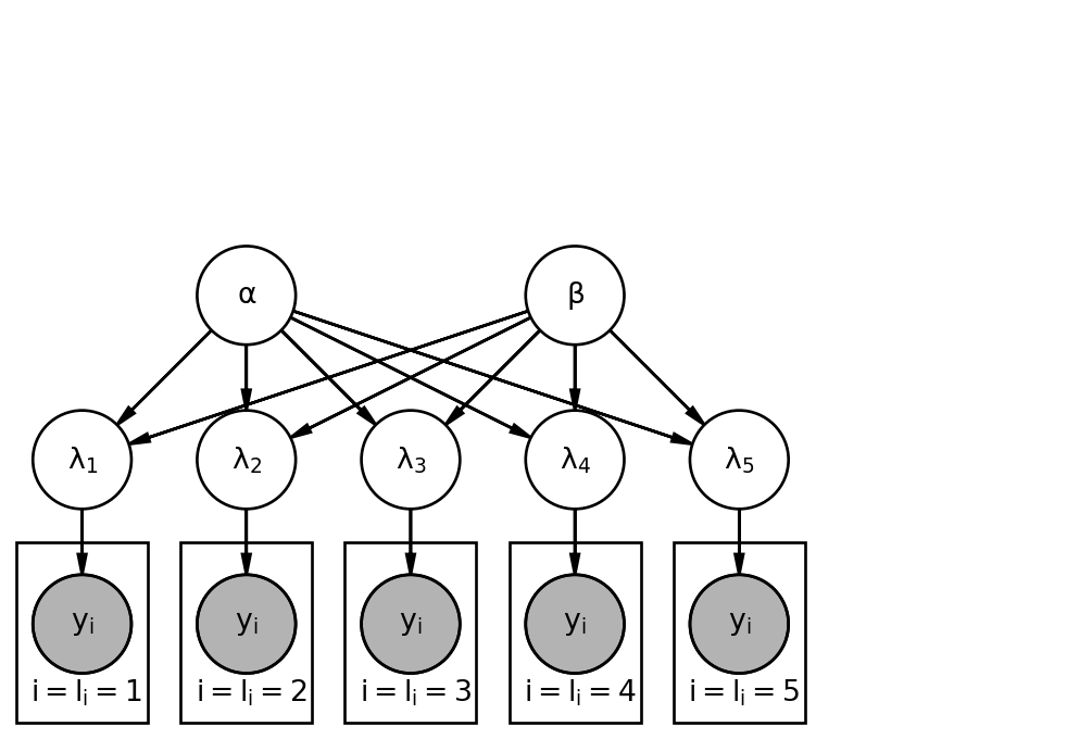
### Graphical Model
The structure of a hierarchical model can be visualized as follows:
- Top Level (Hyperparameters): Independent parameters like $\alpha$ and $\beta$.
- Second Level (Group Parameters): Parameters for each group (e.g., $\lambda_1, \lambda_2, \dots, \lambda_5$) that are dependent on the hyperparameters.
- Lowest Level (Observations): Individual observations (e.g., cookies) are grouped by their respective locations, and their distributions depend on the specific group parameter.
This multi-level structure allows for the estimation of the hyperparameters from the group-specific parameters.
```{python}
#| label: fig-c2l11-hierarchical-model
#| fig-cap: Hierarchical model for chocolate chip cookies
import daft
import matplotlib.pyplot as plt
import warnings
import logging

# Suppress font warnings
warnings.filterwarnings("ignore", category=UserWarning, module="matplotlib.font_manager")

# Also lower logging level for matplotlib font manager
logging.getLogger('matplotlib.font_manager').setLevel(logging.ERROR)

pgm = daft.PGM([6.5, 4.5], node_unit=1.2)

# Hyperparameters
pgm.add_node(daft.Node("alpha", r"$\alpha$", 2, 4));
pgm.add_node(daft.Node("beta", r"$\beta$", 4, 4));

pgm.add_node(daft.Node("lambda_1", r"$\lambda_1$", 1, 3));
pgm.add_node(daft.Node("lambda_2", r"$\lambda_2$", 2, 3));
pgm.add_node(daft.Node("lambda_3", r"$\lambda_3$", 3, 3));
pgm.add_node(daft.Node("lambda_4", r"$\lambda_4$", 4, 3));
pgm.add_node(daft.Node("lambda_5", r"$\lambda_5$", 5, 3));

# Observed data y_i, grouped under lambda_l

pgm.add_node(daft.Node("y_1", r"$y_i$", 1, 2, observed=True));
pgm.add_node(daft.Node("y_2", r"$y_i$", 2, 2, observed=True));
pgm.add_node(daft.Node("y_3", r"$y_i$", 3, 2, observed=True));
pgm.add_node(daft.Node("y_4", r"$y_i$", 4, 2, observed=True));
pgm.add_node(daft.Node("y_5", r"$y_i$", 5, 2, observed=True));

# Edges
pgm.add_edge("alpha", "lambda_1");
pgm.add_edge("alpha", "lambda_2");
pgm.add_edge("alpha", "lambda_3");
pgm.add_edge("alpha", "lambda_4");
pgm.add_edge("alpha", "lambda_5");

pgm.add_edge("beta", "lambda_1");
pgm.add_edge("beta", "lambda_2");
pgm.add_edge("beta", "lambda_3");
pgm.add_edge("beta", "lambda_4");
pgm.add_edge("beta", "lambda_5");

pgm.add_edge("lambda_1", "y_1");
pgm.add_edge("lambda_2", "y_2");
pgm.add_edge("lambda_3", "y_3");
pgm.add_edge("lambda_4", "y_4");
pgm.add_edge("lambda_5", "y_5");

# Plates
pgm.add_plate(daft.Plate([0.6, 1.5, 0.8, 1], label=r"$i=l_i=1$", shift=-0.1));
pgm.add_plate(daft.Plate([1.6, 1.5, 0.8, 1], label=r"$i=l_i=2$", shift=-0.1));
pgm.add_plate(daft.Plate([2.6, 1.5, 0.8, 1], label=r"$i=l_i=3$", shift=-0.1));
pgm.add_plate(daft.Plate([3.6, 1.5, 0.8, 1], label=r"$i=l_i=4$", shift=-0.1));
pgm.add_plate(daft.Plate([4.6, 1.5, 0.8, 1], label=r"$i=l_i=5$", shift=-0.1));


pgm.render()
plt.show()
```
A primary advantage of hierarchical models is their ability to [share information, or borrow strength, from all the data.]{.mark}
- **Indirect Information Sharing**: Even though groups might have their own specific parameters (e.g., your location's $\lambda_1$), the common distribution from which these parameters are drawn means that "information about another location's cookies might provide information about your cookies, at least indirectly."
- **Improved Parameter Estimation**: This shared information leads to more robust and accurate parameter estimates. In the cookie example, "your lambda is not only estimated directly from your 30 cookies, but also indirectly from the other 120 cookies leveraging this hierarchical structure."
The overarching benefit of hierarchical models is their capacity for "Being able to account for relationships in the data while estimating everything with the single model is a primary advantage of using hierarchical models." This provides a flexible and powerful framework for analyzing data with inherent group structures, leading to more realistic and informative inferences.
## Correlations within the Normal hierarchical model :spiral_notepad:
This section is based on the handout titled [Correlation from hierarchical models](handouts/c2l11-correlation-hierarchical-normal-model.pdf) which deep dives into aspects of correlated quantities within hierarchical models by considering the special case of a Normal model.
### Correlated data
In the supplementary material from Module 2, we introduced covariance and correlation.
Recall that [covariance between two random variables is defined as:]{.mark}
$$
\sigma_{xy} = \mathbb{C}ov(X,Y) = \mathbb{E}[(X − \mu_x)(Y − \mu_y)]
$$
where:
- $\mu_x = \mathbb{E}(X)$ and
- $\mu_y = \mathbb{E}(Y)$.
And that [Correlation between X and Y is defined as:]{.mark}
$$
\rho_{xy} = \mathbb{C}or(X,Y) = \frac{\mathbb{C}ov(X,Y)}{\sqrt{\mathbb{V}ar(X) \cdot \mathbb{V}ar(Y)}} = \frac{\sigma_{xy}}{\sqrt{\sigma^2_x \cdot \sigma^2_y}}.
$$
Correlation measures the strength of linear relationship between two variables. Covariance has a useful mathematical property which we will use below.
If $a, b, c, d$ are constants, and $X,Y$ are random variables then
$$
\begin{aligned}
\mathbb{C}ov(a + bX, c + dY) &= \mathbb{C}ov(a, c) + \mathbb{C}ov(a, dY) + \mathbb{C}ov(bX, c) + \mathbb{C}ov(bX, dY) \\
&= \mathbb{C}ov(a,c) + \mathbb{C}ov(a,dY ) + \mathbb{C}ov(bX,c) + \mathbb{C}ov(bX,dY ) \\
&= 0 + 0 + 0 + b \cdot \mathbb{C}ov(X,Y ) \cdot d \\
&= b \cdot d \cdot \sigma_{xy} ,
\end{aligned}
$$
where the 0 terms are due to the fact that constants do not co-vary with anything.
In the examples from this lesson, we use hierarchical models when the data were grouped in some way, so that two observations from the same group were assumed to be more similar than two observations from different groups. [We would therefore expect two observations from the same group to be correlated.]{.mark} It turns out that hierarchical models do correlate such variables, as we will demonstrate with a normal hierarchical model.
### Normal hierarchical model
Suppose our data come from a normal distribution, where each group has its own mean.
In the second stage, we assume that all the group means come from a common normal
distribution.
Let's write this hierarchical model. We $y_{i,j}$ denote the $i$ th observation in group $j$, with mean $\theta_j$. Thus we get:
$$
\begin{aligned}
y_{i,j} \mid \theta_j &\stackrel{iid}{\sim} \mathcal{N}(\theta_j, \sigma^2) \\
\theta_j &\stackrel{iid}{\sim} \mathcal{N}(\mu, \tau^2)
\end{aligned}
$$
where $\sigma^2$, $\tau^2$, and $\mu$ are known constants. To get the marginal distribution of $y_{i,j}$ only, we must compute:
$$
\begin{aligned}
\mathbb{P}r(y_{i,j}) &= \int \mathbb{P}r(y_{i,j}, \theta_j) d\theta_j \\
&= \int \mathbb{P}r(y_{i,j} \mid \theta_j) \mathbb{P}r(\theta_j) d\theta_j
\end{aligned}
$$
With normally distributed variables, it is often easier to work with the following equivalent formulation of the model
$$
\begin{aligned}
\theta_j &= \mu + \nu_j, & \nu_j &\stackrel{iid}{\sim} \mathcal{N}(0, \tau^2) \\
y_{i,j} &= \theta_j + \varepsilon_{i,j}, & \varepsilon_{i,j} &\stackrel{iid}{\sim} \mathcal{N}(0, \sigma^2)
\end{aligned}
$$
with all $\nu_j$ and $\varepsilon_{i,j}$ independent. This allows us to substitute $\theta_j$ into the expression for $y_{i,j}$ to get
$$
y_{i,j} = \mu + \nu_j + \varepsilon_{i,j}.
$$
One nice property of normal random variables is that if $X$ and $Y$ are both normally distributed (correlated or uncorrelated), then the new variable $X + Y$ will also be normally distributed. Hence $\mathbb{P}r(y_{i,j})$ is a normal distribution with mean
$$
\begin{aligned}
\mathbb{E}(y_{i,j}) &= \mathbb{E}(\mu + \nu_j + \varepsilon_{i,j}) \\
&= E(\mu) + E(\nu_j) + E(\varepsilon_{i,j}) \\
&= \mu + 0 + 0 \\
&= \mu
\end{aligned}
$$
and variance
$$
\begin{aligned}
\mathbb{V}ar(y_{i,j}) =& \mathbb{V}ar(\mu + \nu_j + \varepsilon_{i,j} ) \\
=& \mathbb{C}ov(\mu + \nu_j + \varepsilon_{i,j} , \mu + \nu_j + \varepsilon_{i,j} ) \\
=& \mathbb{C}ov(\mu,\mu) + \mathbb{C}ov(\nu_j ,\nu_j ) + \mathbb{C}ov(\varepsilon_{i,j} ,\varepsilon_{i,j} ) \\
& + 2 \cdot \mathbb{C}ov(\mu,\nu_j ) + 2 \cdot \mathbb{C}ov(\mu,\varepsilon_{i,j} ) \\
& + 2 \cdot \mathbb{C}ov(\nu_j ,\varepsilon_{i,j} ) \\
=& 0 + \mathbb{V}ar(\nu_j ) + \mathbb{V}ar(\varepsilon_{i,j} ) + 0 + 0 + 0 &&& \text{(since } \nu_j \text{ and } \varepsilon_{i,j} \text{ are independent)} \\
=& \tau^2 + \sigma^2 .
\end{aligned}
$$
Now, we want to show that observations in the same group are correlated under this
hierarchical model.
Let's take, for example, observations 1 and 2 from group $j, y_{1,j}$ and $y_{2,j}$.
It does not matter which two you select, as long as they are from the same group. We know that $\mathbb{V}ar(y_{1,j}) = \mathbb{V}ar(y_{2,j}) = \tau^2 + \sigma^2$. What about their covariance?
$$
\begin{aligned}
\mathbb{C}ov(y_{1,j},y_{2,j}) &= \mathbb{C}ov(\mu + \nu_j + \varepsilon_{2,j}, \mu + \nu_j + \varepsilon_{2,j}) \\
&= \mathbb{C}ov(\mu,\mu) + \mathbb{C}ov(\nu_j,\nu_j)
+ \mathbb{C}ov(\varepsilon_{1,j},\varepsilon_{2,j})
+ 2 \cdot \mathbb{C}ov(\mu,\nu_j)
+ \mathbb{C}ov(\mu,\varepsilon_{1,j})
+ \mathbb{C}ov(\mu,\varepsilon_{2,j})
+ \mathbb{C}ov(\nu_j,\varepsilon_{1,j})
+ \mathbb{C}ov(\nu_j,\varepsilon_{2,j}) \\
&= 0 + \mathbb{V}ar(\nu_j) + 0
+ 2 \cdot 0
+ 0 + 0 + 0
+ 0 \qquad \text{(as } \varepsilon_{1,j} \text{ and } \varepsilon_{2,j} \text{ are independent)}
&= \tau^2
\end{aligned}
$$
which gives us correlation:
$$
\begin{aligned}
\mathbb{C}or(y_{1,j},y_{2,j}) &= \mathbb{C}ov(y_{1,j},y_{2,j})/\sqrt{\mathbb{V}ar(y_{1,j}) \cdot \mathbb{V}ar(y_{2,j})} \\
&= \tau^2/\sqrt{(\tau^2 + \sigma^2) \cdot (\tau^2 + \sigma^2)} \\
&= \tau^2/\sqrt{(\tau^2 + \sigma^2) \cdot (\tau^2 + \sigma^2)} \\
&= \tau^2/\sqrt{(\tau^2 + \sigma^2)^2} \\
&= \frac{\tau^2}{\tau^2 + \sigma^2}.
\end{aligned}
$$
Finally, let's check the covariance between observations in different groups. Let’s take observation $i$ from groups 1 and 2 (again, our choices do not matter), $y_{i,1}$ and $y_{i,2}$.
Their covariance is
$$
\begin{aligned}
\mathbb{C}ov(y_{i,1},y_{i,2}) &= \mathbb{C}ov(\mu + \nu_1 + \varepsilon_{i,1}, \mu + \nu_2 + \varepsilon_{i,2}) \\
&= \mathbb{C}ov(\mu,\mu) + \mathbb{C}ov(\nu_1,\nu_2) + \mathbb{C}ov(\varepsilon_{i,1},\varepsilon_{i,2}) \\
&\quad + \mathbb{C}ov(\mu,\nu_1) + \mathbb{C}ov(\mu,\nu_2) + \mathbb{C}ov(\mu,\varepsilon_{i,1}) + \mathbb{C}ov(\mu,\varepsilon_{i,2}) \\
&\quad + \mathbb{C}ov(\nu_1,\varepsilon_{i,1}) + \mathbb{C}ov(\nu_2,\varepsilon_{i,2}) \\
&= 0 + 0 + 0 + 0 + 0 + 0 + 0 + 0 + 0 \qquad \text{(as all } \varepsilon \text{ and } \nu \text{ are independent)} \\
&= 0,
\end{aligned}
$$
which obviously yields correlation 0.
[Thus, we have demonstrated that observations from the same group are correlated while observations from different groups are uncorrelated in the marginal distribution for observations.]{.mark}
## Applications of hierarchical modeling
Handout: [Common applications of Bayesian hierarchical models](handouts/c2l11-hierarchical-model-applications.pdf)
## Prior predictive simulation
### Data
Let's fit our hierarchical model for counts of chocolate chips. The data can be found in `cookies.dat`.
```{r}
#| label: load-cookies-data
dat = read.table(file="data/cookies.dat", header=TRUE)
head(dat)
```
```{r}
#| label: cookies-data-summary
table(dat$location)
```
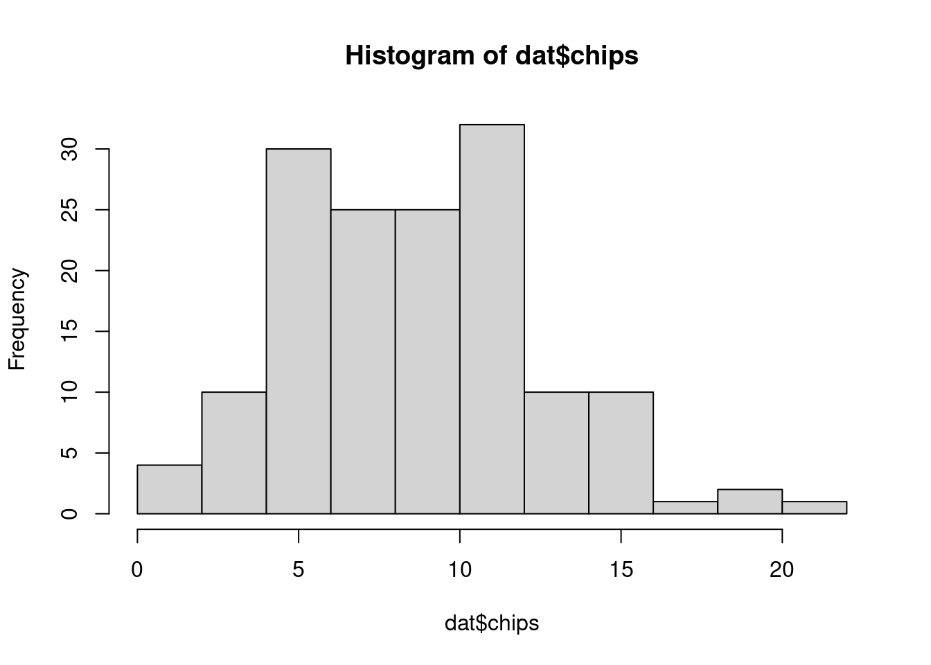
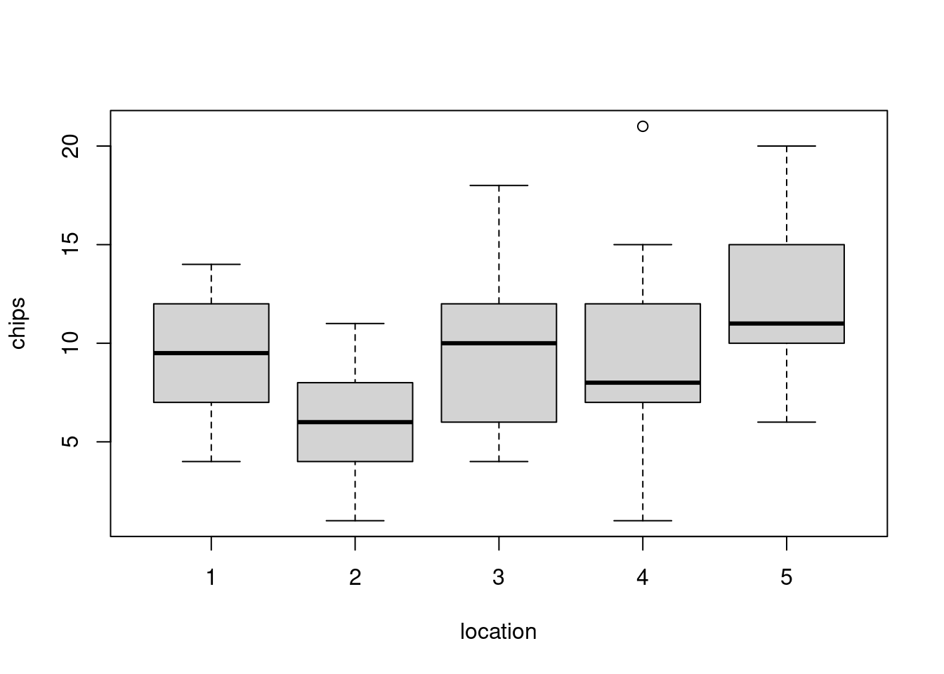
We can also visualize the distribution of chips by location.
```{r}
#| label: fig-cookies-data-hist
hist(dat$chips)
```
```{r}
#| label: fig-cookies-data-boxplot
boxplot(chips ~ location, data=dat)
```
### Prior predictive checks {#sec-c2l11-prior-predictive-checks}
Before implementing the model, we need to select prior distributions for $\alpha$ and $\beta$, the hyperparameters governing the gamma distribution for the $\lambda$ parameters. First, think about what the $\lambda$'s represent. For location $j$, $\lambda_j$ is the expected number of chocolate chips per cookie. Hence, $\alpha$ and $\beta$ control the distribution of these means between locations. The mean of this gamma distribution will represent the overall mean of number of chips for all cookies. The variance of this gamma distribution controls the variability between locations. If this is high, the mean number of chips will vary widely from location to location. If it is small, the mean number of chips will be nearly the same from location to location.
To see the effects of different priors on the distribution of $\lambda$'s, we can simulate. Suppose we try independent exponential priors for $\alpha$ and $\beta$.
```{r}
#| label: lst-prior-sim-1
set.seed(112)
n_sim = 500
alpha_pri = rexp(n_sim, rate=1.0/2.0)
beta_pri = rexp(n_sim, rate=5.0)
mu_pri = alpha_pri/beta_pri
sig_pri = sqrt(alpha_pri/beta_pri^2)

summary(mu_pri)
```
```{r}
#| label: lst-prior-sim-2
summary(sig_pri)
```
After simulating from the priors for $\alpha$ and $\beta$, we can use those samples to simulate further down the hierarchy:
```{r}
#| label: lst-prior-sim-3
lam_pri = rgamma(n=n_sim, shape=alpha_pri, rate=beta_pri)
summary(lam_pri)
```
Or for a prior predictive reconstruction of the original data set:
```{r}
#| label: lst-prior-sim-4
(lam_pri = rgamma(n=5, shape=alpha_pri[1:5], rate=beta_pri[1:5]))
```
```{r}
#| label: lst-prior-sim-5
(y_pri = rpois(n=150, lambda=rep(lam_pri, each=30)))
```
Because these priors have high variance and are somewhat noninformative, they produce unrealistic predictive distributions. Still, enough data would overwhelm the prior, resulting in useful posterior distributions. Alternatively, we could tweak and simulate from these prior distributions until they adequately represent our prior beliefs. Yet another approach would be to re-parameterize the gamma prior, which we'll demonstrate as we fit the model.
## JAGS Model
```{r}
#| label: load-rjags
library("rjags")
```
```{r}
#| label: cookies-model-string
mod_string = " model {
for (i in 1:length(chips)) {
  chips[i] ~ dpois(lam[location[i]])
}

for (j in 1:max(location)) {
  lam[j] ~ dgamma(alpha, beta)
}

alpha = mu^2 / sig^2
beta = mu / sig^2

mu ~ dgamma(2.0, 1.0/5.0)
sig ~ dexp(1.0)

} "

set.seed(113)

data_jags = as.list(dat)

params = c("lam", "mu", "sig")

mod = jags.model(textConnection(mod_string), data=data_jags, n.chains=3)
update(mod, 1e3)

mod_sim = coda.samples(model=mod,
                       variable.names=params,
                       n.iter=5e3)
mod_csim = as.mcmc(do.call(rbind, mod_sim))
```
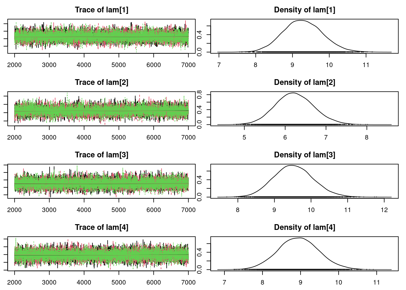
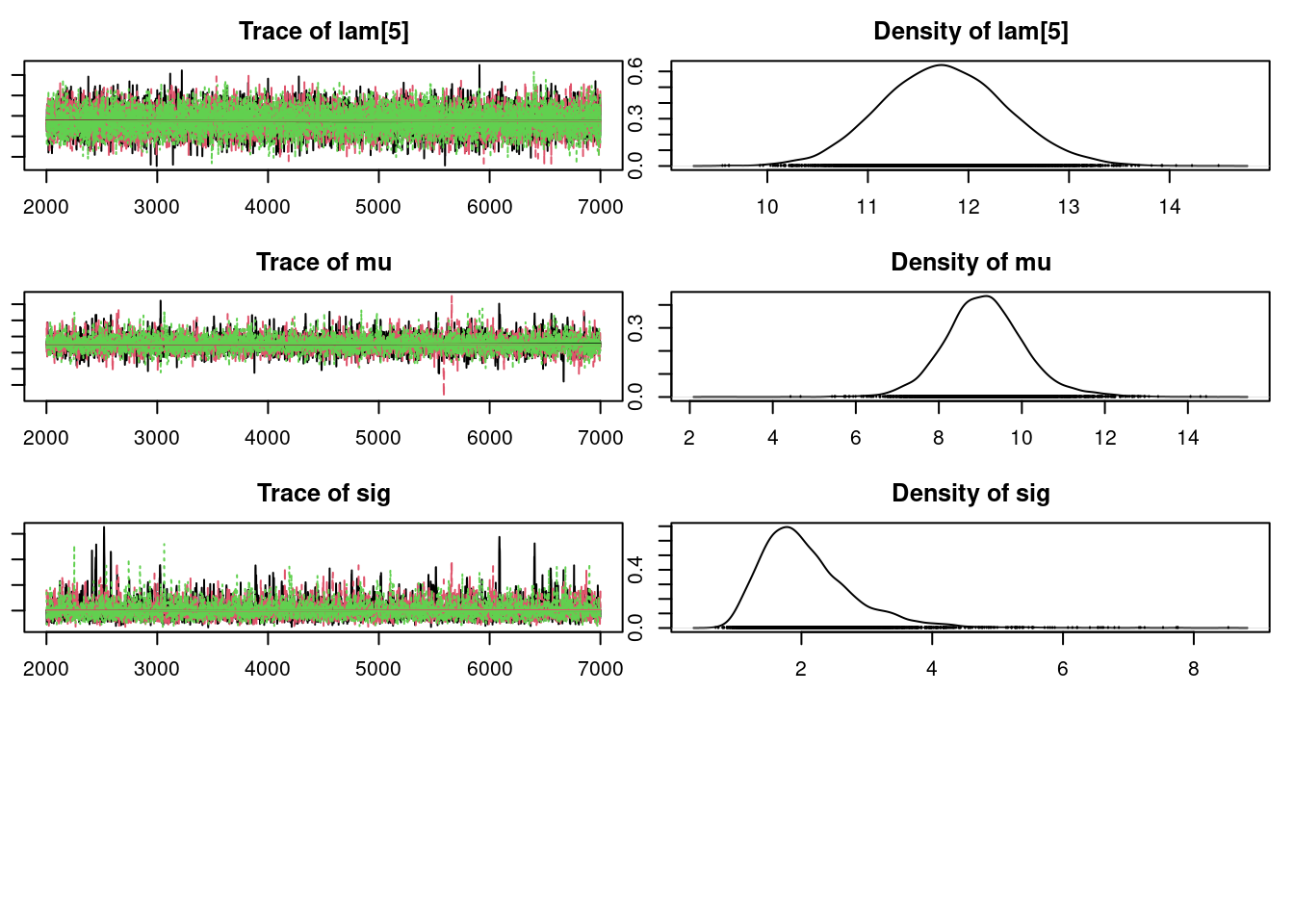
```{r}
#| label: fig-cookies-convergence
## convergence diagnostics
par(mar = c(2.5, 1, 2.5, 1))
plot(mod_sim)
```
```{r}
#| label: fig-cookies-convergence-diagnostics
gelman.diag(mod_sim)
autocorr.diag(mod_sim)
```
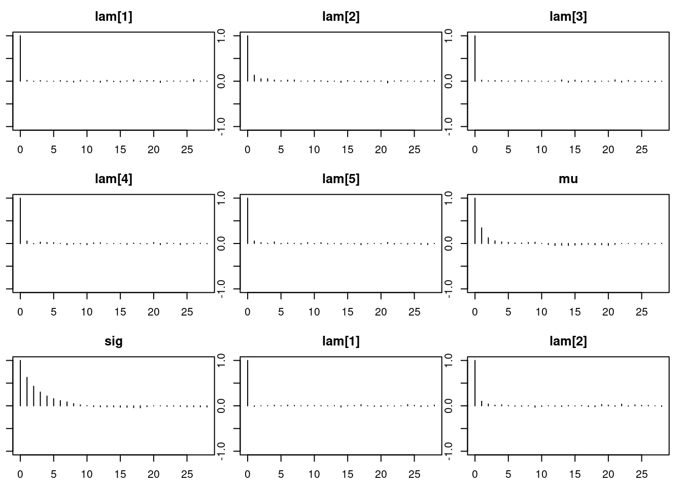
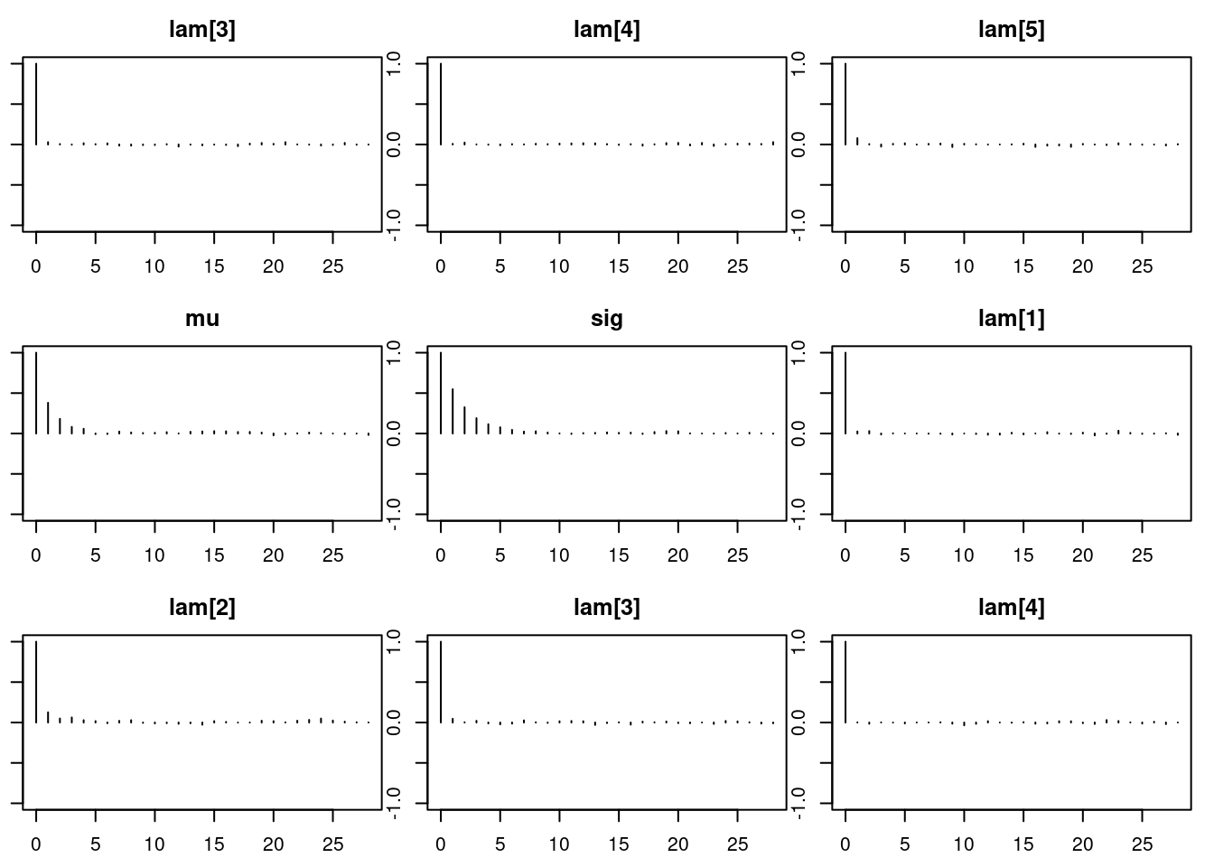
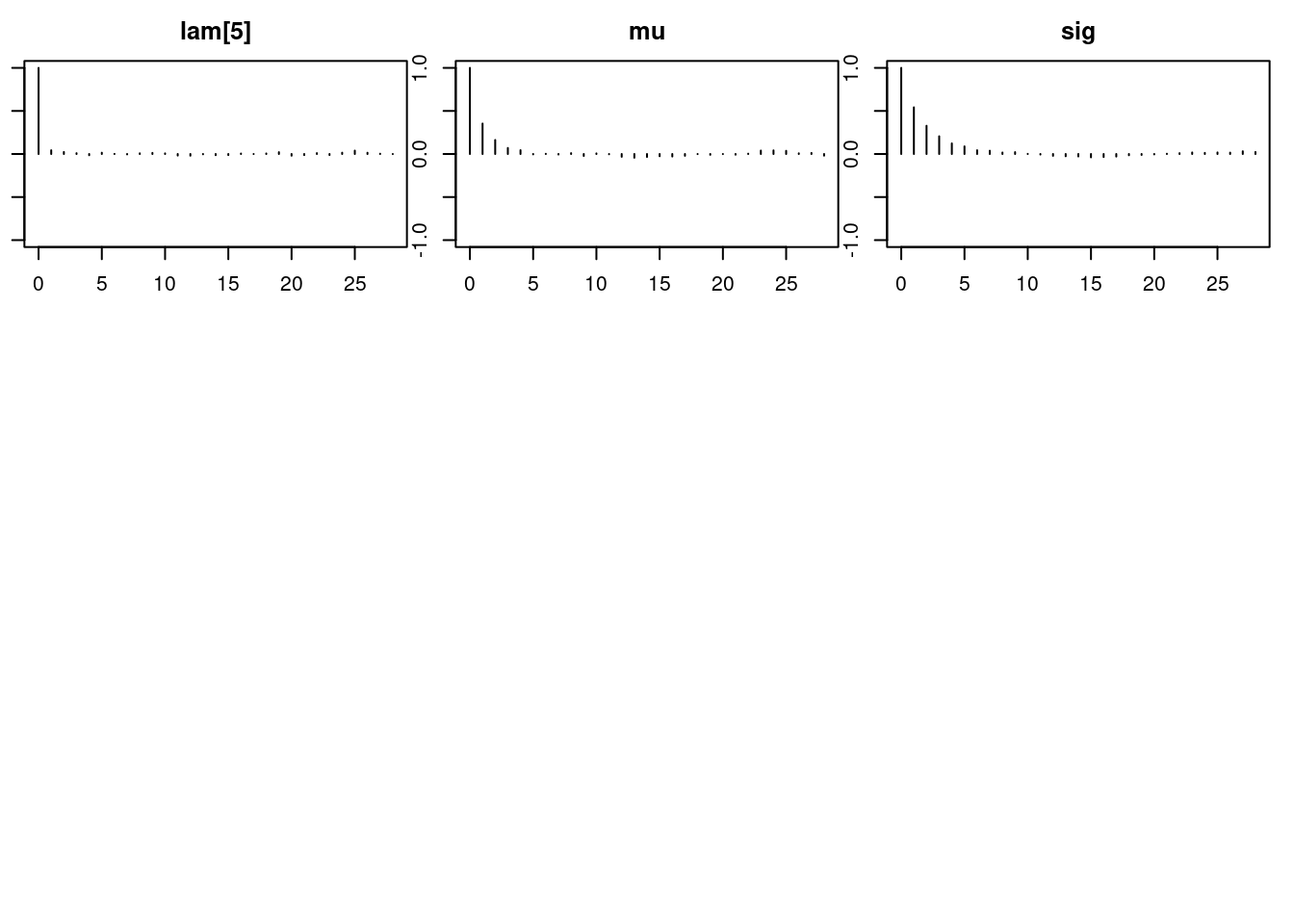
```{r}
#| label: fig-cookies-autocorr
#| layout-ncol: 3
par(mar = c(2.5, 1, 2.5, 1))
autocorr.plot(mod_sim)
```
```{r}
#| label: fig-cookies-effective-sample-size
effectiveSize(mod_sim)
## compute DIC
dic = dic.samples(mod, n.iter=1e3)
```
\index{model selection!DIC}
### Model checking
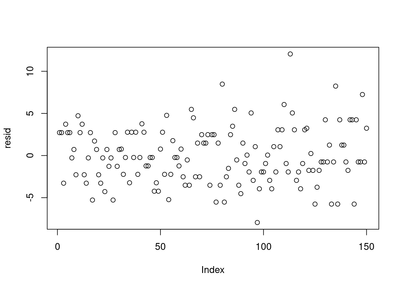
After assessing convergence, we can check the fit via residuals. With a hierarchical model, there are now two levels of residuals: the observation level and the location mean level. To simplify, we'll look at the residuals associated with the posterior means of the parameters.
First, we have observation residuals, based on the estimates of location means.
```{r}
#| label: lst-cookies-observation-residuals
## observation level residuals
(pm_params = colMeans(mod_csim))
```
```{r}
#| label: fig-cookies-observation-residuals
yhat = rep(pm_params[1:5], each=30)
resid = dat$chips - yhat
plot(resid)
```
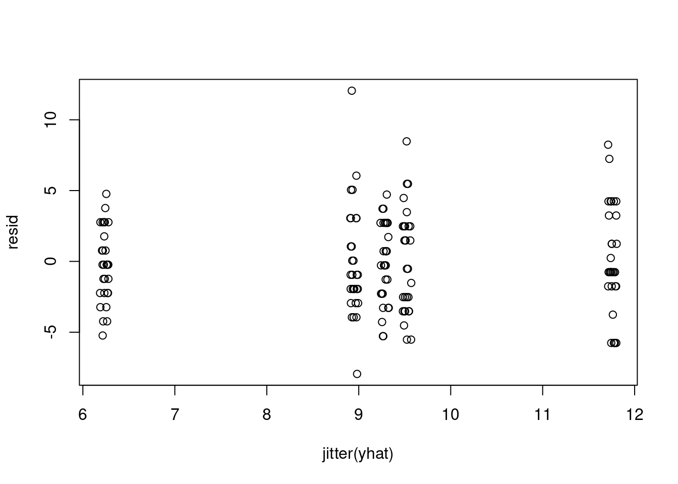
```{r}
#| label: fig-cookies-observation-residuals-jitter
plot(jitter(yhat), resid)
```
```{r}
#| label: lst-cookies-observation-residuals-var
var(resid[yhat<7])
```
```{r}
#| label: lst-cookies-observation-residuals-var2
var(resid[yhat>11])
```
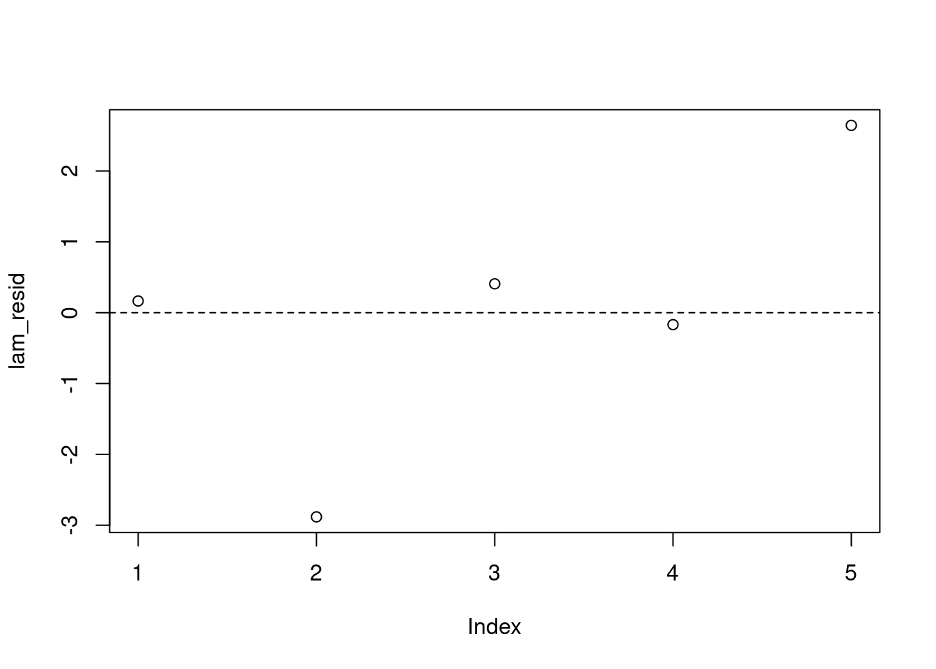
Also, we can look at how the location means differ from the overall mean $\mu$.
```{r}
#| label: lst-cookies-location-residuals
## location level residuals
lam_resid = pm_params[1:5] - pm_params["mu"]
plot(lam_resid)
abline(h=0, lty=2)
```
We don't see any obvious violations of our model assumptions.
### Results
```{r}
#| label: cookies-model-summary
summary(mod_sim)
```
## Posterior predictive simulation
\index{MCMC!posterior predictive simulation}
Just as we did with the prior distribution, we can use these posterior samples to get Monte Carlo estimates that interest us from the posterior predictive distribution.
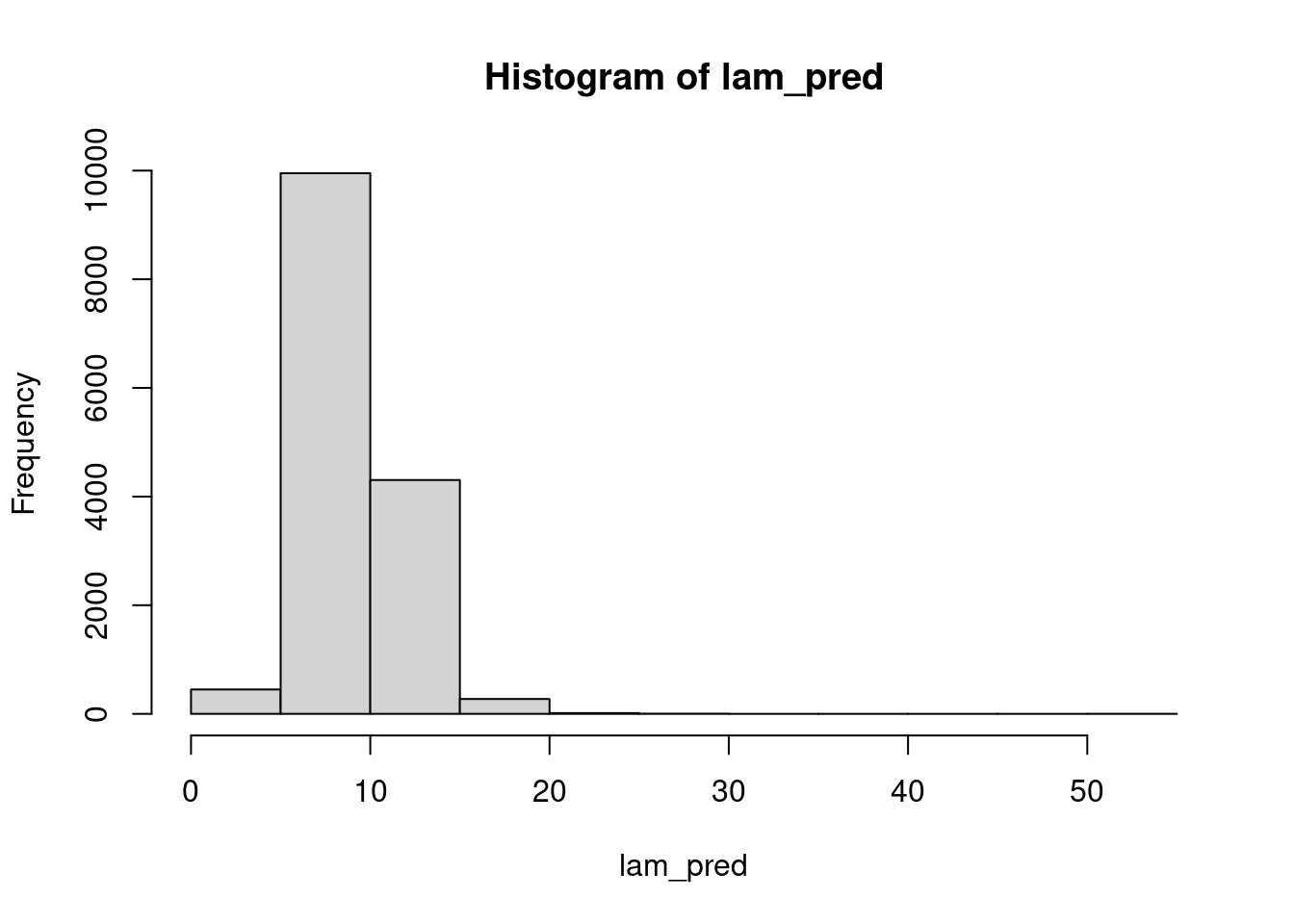
For example, we can use draws from the posterior distribution of $\mu$ and $\sigma$ to simulate the posterior predictive distribution of the mean for a new location.
```{r}
#| label: lst-cookies-posterior-predictive
(n_sim = nrow(mod_csim))
```
```{r}
#| label: fig-cookies-lambda-prediction
lam_pred = rgamma(n=n_sim, shape=mod_csim[,"mu"]^2/mod_csim[,"sig"]^2,
                  rate=mod_csim[,"mu"]/mod_csim[,"sig"]^2)
hist(lam_pred)
```
```{r}
#| label: lst-cookies-lambda-prediction-mean
mean(lam_pred > 15)
```
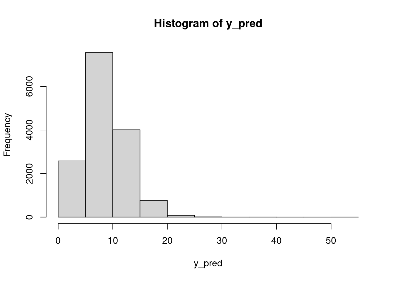
Using these $\lambda$ draws, we can go to the observation level and simulate the number of chips per cookie, which takes into account the uncertainty in $\lambda$:
```{r}
#| label: lst-cookies-predicted-chips
y_pred = rpois(n=n_sim, lambda=lam_pred)
hist(y_pred)
```
```{r}
#| label: lst-cookies-predicted-chips-mean
mean(y_pred > 15)
```
```{r}
#| label: fig-cookies-predicted-chips-hist
hist(dat$chips)
```
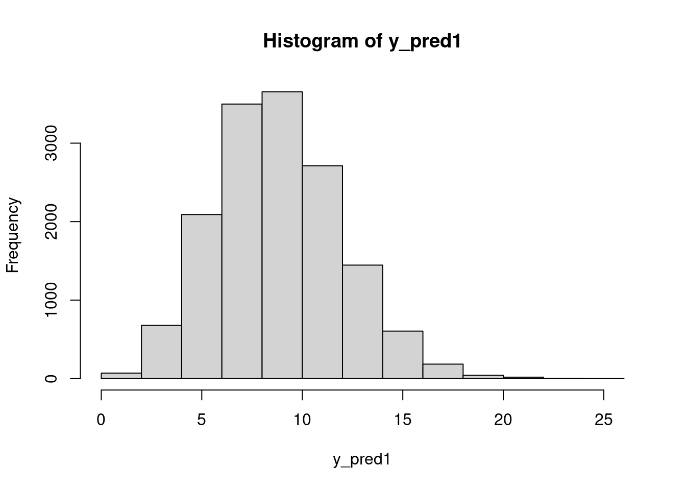
Finally, we could answer questions like: what is the posterior probability that the next cookie produced in Location 1 will have fewer than seven chips?
```{r}
#| label: fig-hist-cookies-predicted-chips-location1
y_pred1 = rpois(n=n_sim, lambda=mod_csim[,"lam[1]"])
hist(y_pred1)
```
```{r}
#| label: lst-cookies-predicted-chips-location1
mean(y_pred1 < 7)
```
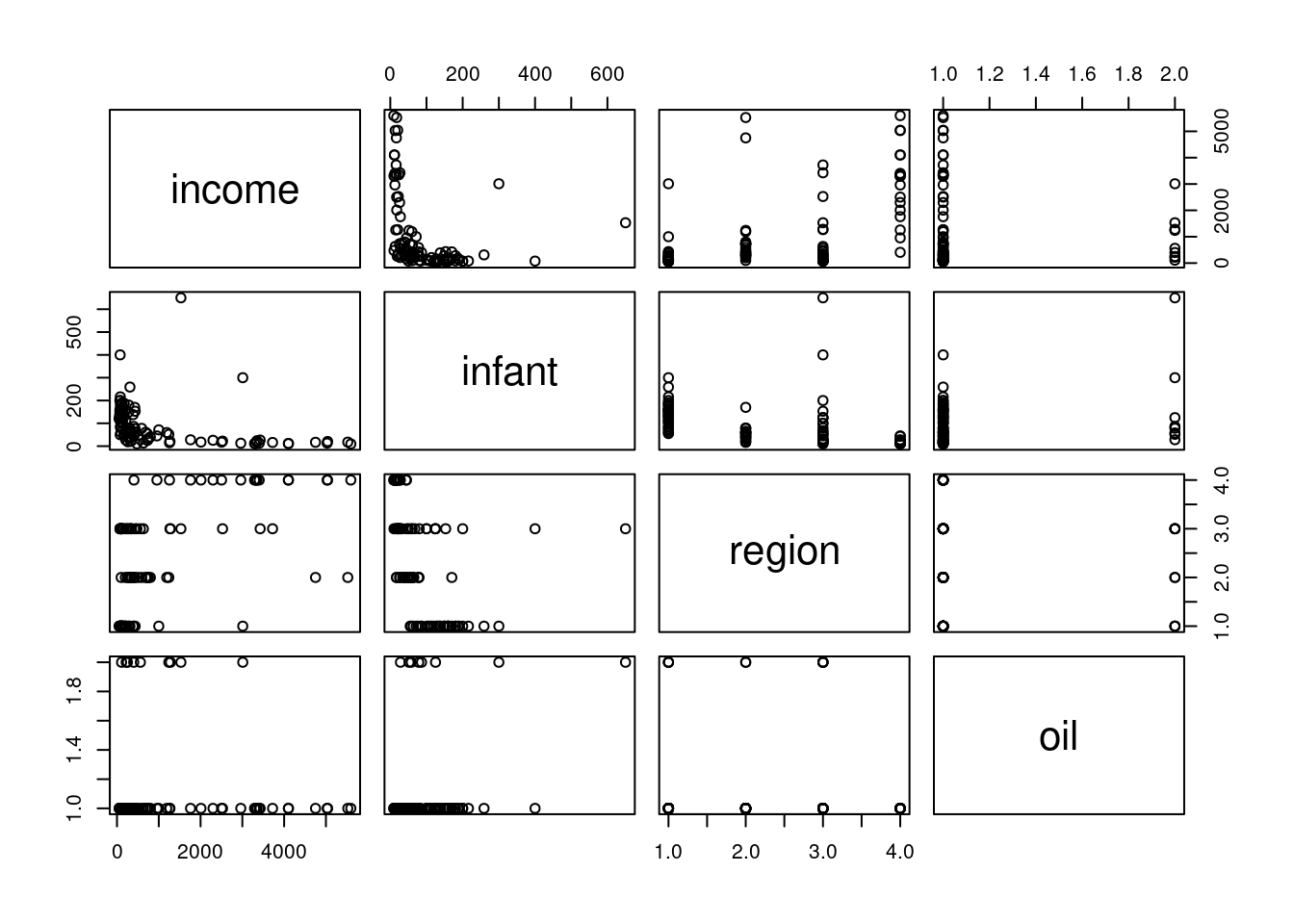
## Random intercept linear model
\index{dataset!Leinhardt}
\index{model!{random intercept}}
We can extend the linear model for the Leinhardt data on infant mortality by incorporating the `region` variable. We'll do this with a hierarchical model, where each region has its own intercept.
```{r}
#| label: load-leinhardt-data
library("car")
data("Leinhardt")
?Leinhardt
str(Leinhardt)
```
```{r}
#| label: fig-leinhardt-pairs-plot
pairs(Leinhardt)
```
```{r}
#| label: fig-leinhardt-head
head(Leinhardt)
```
Previously, we worked with infant mortality and income on the logarithmic scale. Recall also that we had to remove some missing data.
```{r}
#| label: lst-leinhardt-data-preparation
dat = na.omit(Leinhardt)
dat$logincome = log(dat$income)
dat$loginfant = log(dat$infant)
str(dat)
```
Now we can fit the proposed model:
```{r}
#| label: lst-leinhardt-load-rjags
library("rjags")
```
```{r}
#| label: leinhardt-model-string
mod_string = " model {
  for (i in 1:length(y)) {
    y[i] ~ dnorm(mu[i], prec)
    mu[i] = a[region[i]] + b[1]*log_income[i] + b[2]*is_oil[i]
  }

  for (j in 1:max(region)) {
    a[j] ~ dnorm(a0, prec_a)
  }

  a0 ~ dnorm(0.0, 1.0/1.0e6)
  prec_a ~ dgamma(1/2.0, 1*10.0/2.0)
  tau = sqrt( 1.0 / prec_a )

  for (j in 1:2) {
    b[j] ~ dnorm(0.0, 1.0/1.0e6)
  }

  prec ~ dgamma(5/2.0, 5*10.0/2.0)
  sig = sqrt( 1.0 / prec )
} "
```
```{r}
#| label: lst-leinhardt-data-jags
set.seed(116)
data_jags = list(y=dat$loginfant, log_income=dat$logincome,
                  is_oil=as.numeric(dat$oil=="yes"), region=as.numeric(dat$region))
data_jags$is_oil
table(data_jags$is_oil, data_jags$region)
params = c("a0", "a", "b", "sig", "tau")

mod = jags.model(textConnection(mod_string), data=data_jags, n.chains=3)
update(mod, 1e3) # burn-in
mod_sim = coda.samples(model=mod,
variable.names=params,
n.iter=5e3)
mod_csim = as.mcmc(do.call(rbind, mod_sim)) # combine multiple chains
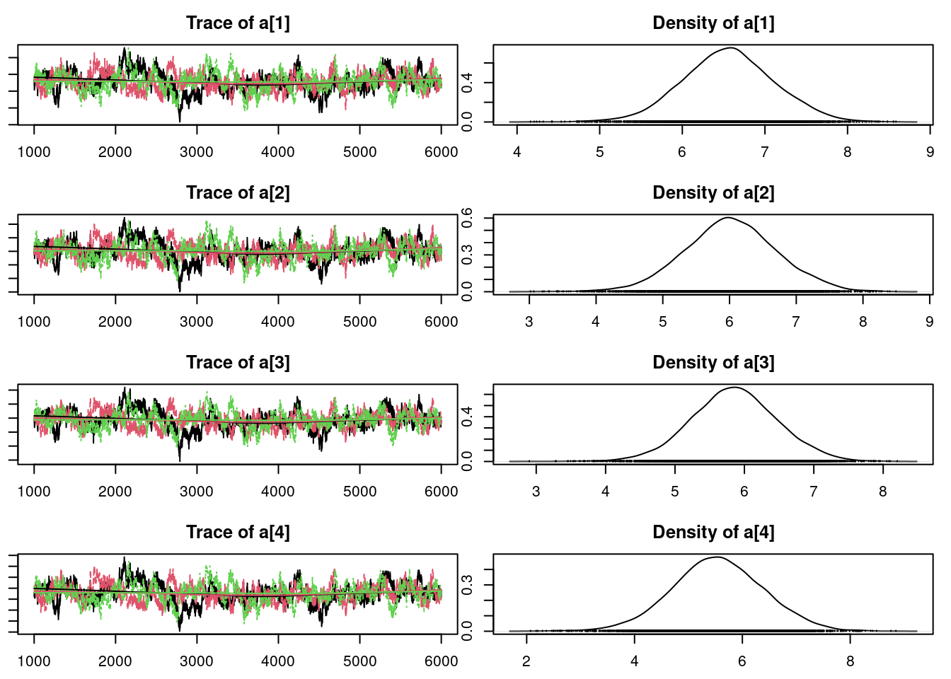
## convergence diagnostics
par(mar = c(2.5, 1, 2.5, 1))
plot(mod_sim)
gelman.diag(mod_sim)
autocorr.diag(mod_sim)
autocorr.plot(mod_sim)
effectiveSize(mod_sim)
```
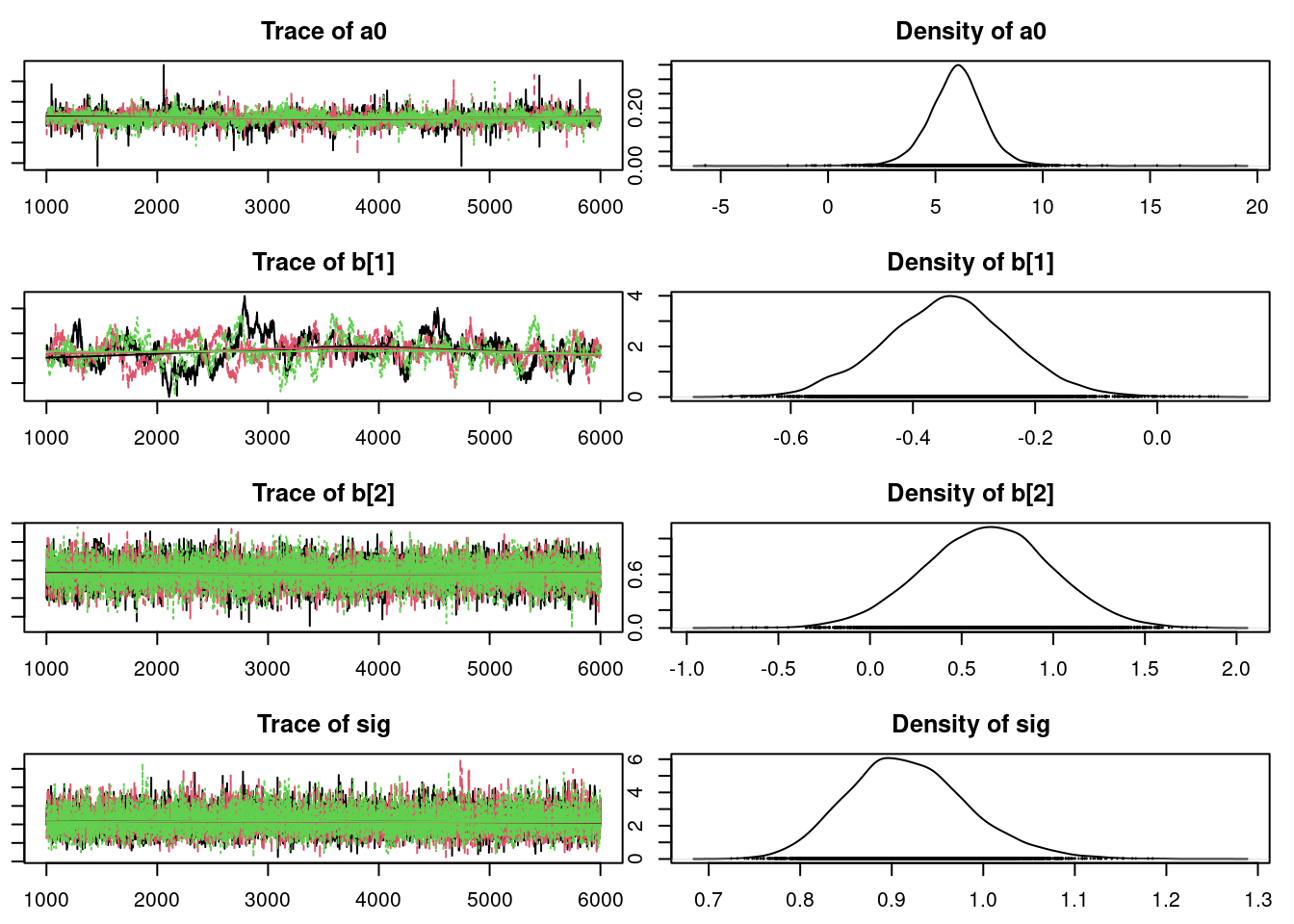
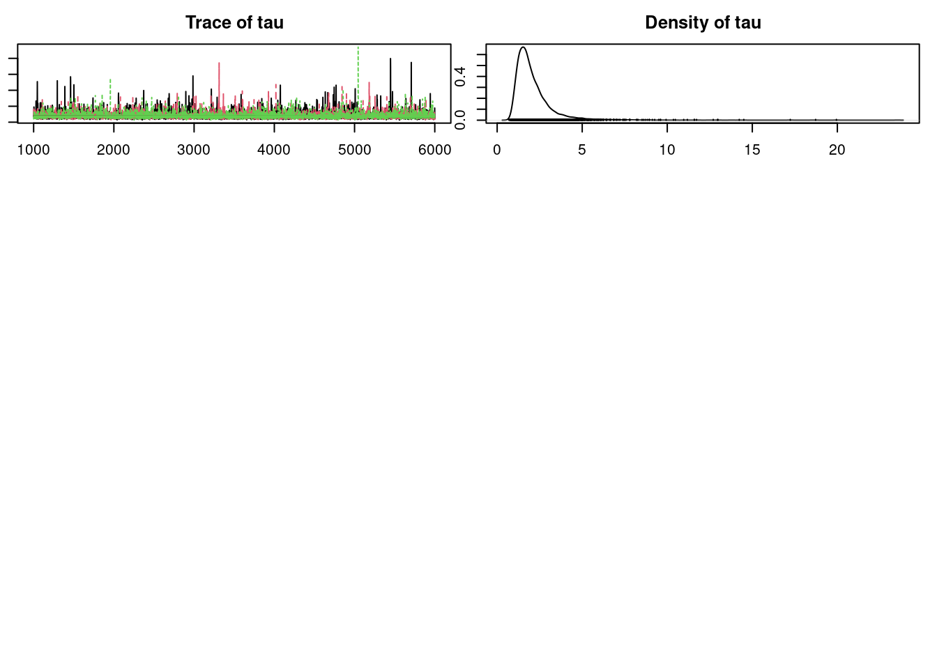
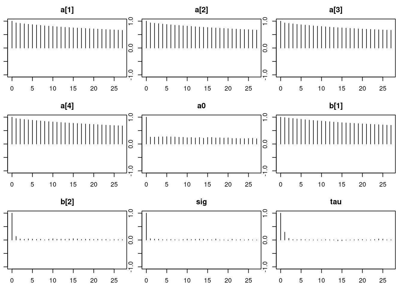
### Results
Convergence looks okay, so let's compare this with the old model from Lesson 7 using DIC:
```{r}
#| label: lst-leinhardt-dic
dic.samples(mod, n.iter=1e3)
### nonhierarchical model: 230.1
```
It appears that this model is an improvement over the non-hierarchical one we fit earlier. Notice that the penalty term, which can be interpreted as the "effective" number of parameters, is less than the actual number of parameters (nine). There are fewer "effective" parameters because they are "sharing" information or "borrowing strength" from each other in the hierarchical structure. If we had skipped the hierarchy and fit one intercept, there would have been four parameters. If we had fit separate, independent intercepts for each region, there would have been seven parameters (which is close to what we ended up with).
Finally, let's look at the posterior summary.
```{r}
#| label: lst-leinhardt-model-summary
summary(mod_sim)
```
In this particular model, the intercepts do not have a real interpretation because they correspond to the mean response for a country that does not produce oil and has USD0 log-income per capita (which is USD1 income per capita). We can interpret $a_0$ as the overall mean intercept and $\tau$ as the standard deviation of intercepts across regions.
### Other models
\index{Deviance information criterion} \index{model selection!DIC}
We have not investigated adding interaction terms, which might be appropriate. We only considered adding hierarchy on the intercepts, but in reality nothing prevents us from doing the same for other terms in the model, such as the coefficients for income and oil. We could try any or all of these alternatives and see how the DIC changes for those models. This, together with other model checking techniques we have discussed could be used to identify your *best* model that you can use to make inferences and predictions.
## Mixture models
Histograms of data often reveal that they do not follow any standard probability distribution. Sometimes we have explanatory variables (or covariates) to account for the different values, and normally distributed errors are adequate, as in normal regression. However, if we only have the data values themselves and no covariates, we might have to fit a non-standard distribution to the data. One way to do this is by mixing standard distributions.
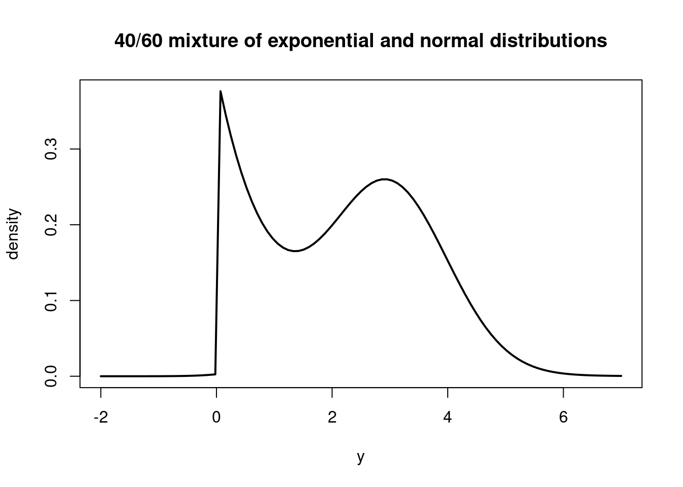
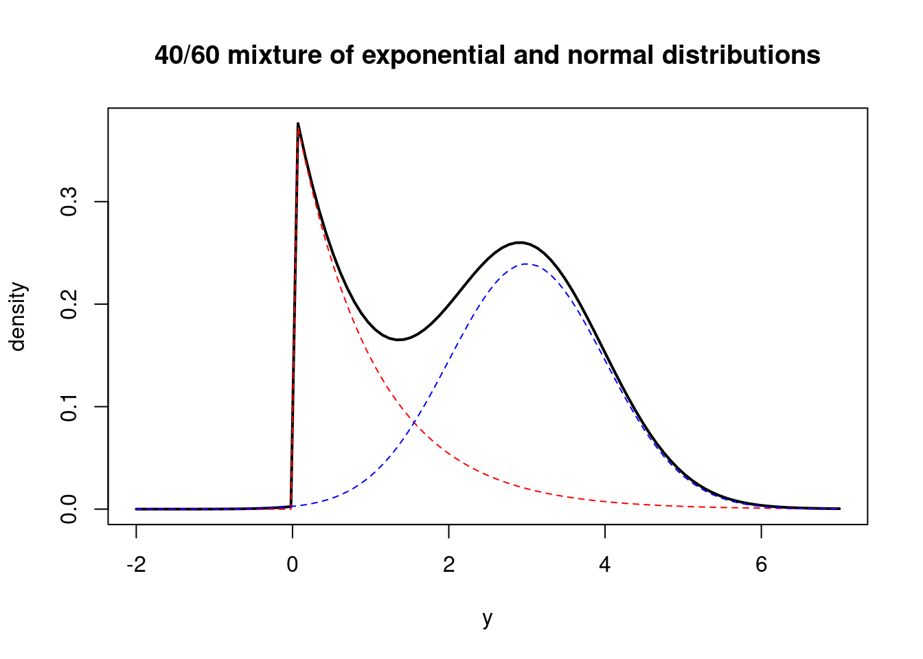
Mixture distributions are just a weighted combination of probability distributions. For example, we could take an exponential distribution with mean 1 and normal distribution with mean 3 and variance 1 (although typically the two mixture components would have the same support; here the exponential component has to be non-negative and the normal component can be positive or negative). Suppose we give them weights: 0.4 for the exponential distribution and 0.6 for the normal distribution. We could write the PDF for this distribution as
$$
\mathbb{P}r(y) = 0.4 \cdot \exp(-y) \cdot \mathbb{I}_{(y \ge 0)} + 0.6 \cdot \frac{1}{\sqrt{2 \pi}} \exp\left(- \frac{1}{2} (y - 3)^2\right)
$$ {#eq-c2l11-mixture-1-pdf}
where $\mathbb{I}_{(y \ge 0)}$ is the indicator function that is 1 if $y \ge 0$ and 0 otherwise. This PDF is a mixture of the exponential and normal distributions, with the weights indicating the relative contribution of each distribution to the overall PDF.
The PDF of this mixture distribution would look like this:
```{r}
#| label: fig-mixture-distribution
curve( 0.4*dexp(x, 1.0) + 0.6*dnorm(x, 3.0, 1.0), from=-2.0, to=7.0, ylab="density", xlab="y", main="40/60 mixture of exponential and normal distributions", lwd=2)
```
We could think of these two distributions as governing two distinct populations, one following the exponential distribution and the other following the normal distribution.
Let's draw the weighted PDFs for each population.
```{r}
#| label: fig-mixture-distribution-pdfs
curve( 0.4*dexp(x, 1.0) + 0.6*dnorm(x, 3.0, 1.0), from=-2.0, to=7.0, ylab="density", xlab="y", main="40/60 mixture of exponential and normal distributions", lwd=2)
curve( 0.4*dexp(x, 1.0), from=-2.0, to=7.0, col="red", lty=2, add=TRUE)
curve( 0.6*dnorm(x, 3.0, 1.0), from=-2.0, to=7.0, col="blue", lty=2, add=TRUE)
```
The general form for a discrete mixture of distributions is as follows:
$$
\mathbb{P}r(y) = \sum_{j=1}^J \omega_j \cdot f_j (y)
$$ {#eq-c2l11-mixture-2-pdf}
where the $\omega$'s are positive weights that add up to 1 (they are probabilities) and each of the $J$ $f_j(y)$ functions is a PDF for some distribution. In the example above, the weights were 0.4 and 0.6, $f_1$ was an exponential PDF and $f_2$ was a normal PDF.
One way to simulate from a mixture distribution is with a hierarchical model. We first simulate an indicator for which "population" the next observation will come from using the weights $\omega$. Let's call this $z_i$. In the example above, $z_i$ would take the value 1 (indicating the exponential distribution) with probability 0.4 and 2 (indicating the normal distribution) with probability 0.6. Next, simulate the observation $y_i$ from the distribution corresponding to $z_i$.
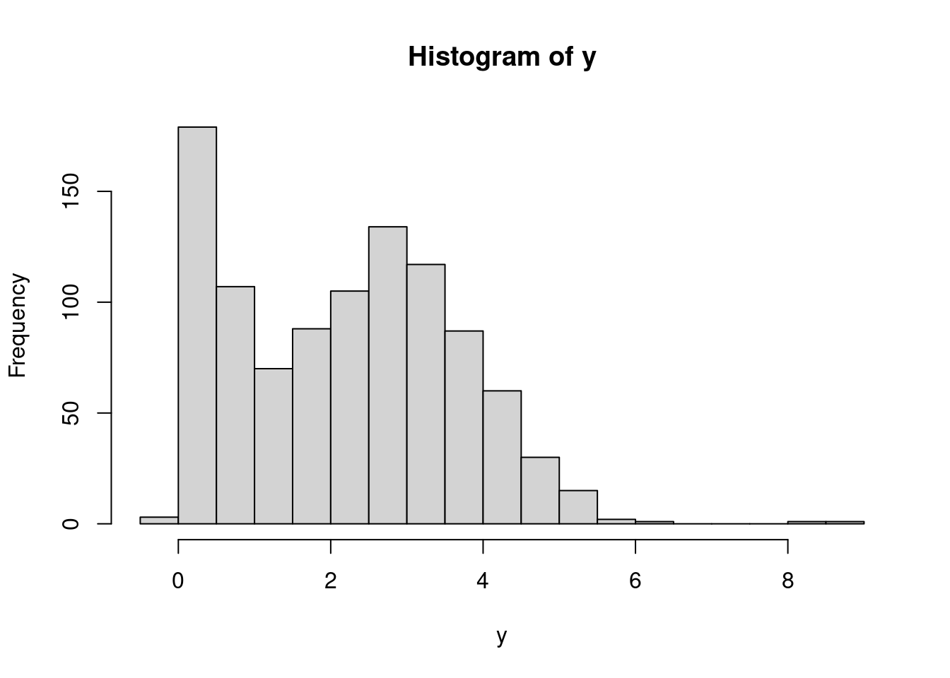
Let's simulate from our example mixture distribution.
```{r}
set.seed(117)
n = 1000
z = numeric(n)
y = numeric(n)
for (i in 1:n) {
  z[i] = sample.int(2, 1, prob=c(0.4, 0.6)) # returns a 1 with probability 0.4, or a 2 with probability 0.6
  if (z[i] == 1) {
    y[i] = rexp(1, rate=1.0)
  } else if (z[i] == 2) {
    y[i] = rnorm(1, mean=3.0, sd=1.0)
  }
}
hist(y, breaks=30)
```
If we keep only the $y$ values and throw away the $z$ values, we have a sample from the mixture model above. To see that they are equivalent, we can marginalize the joint distribution of $y$ and $z$:
$$
\begin{aligned}
\mathbb{P}r(y) &= \sum_{j=1}^2 \mathbb{P}r(y, z=j) \\
&= \sum_{j=1}^2 \mathbb{P}r(z=j) \cdot \mathbb{P}r(y \mid z=j) \\
&= \sum_{j=1}^2 \omega_j \cdot f_j(y)
\end{aligned}
$$ {#eq-c2l11-mixture-3-pdf}
### Bayesian inference for mixture models
When we fit a mixture model to data, we usually only have the $y$ values and do not know which "population" they belong to. Because the $z$ variables are unobserved, they are called *latent* variables. We can treat them as parameters in a hierarchical model and perform Bayesian inference for them. The hierarchial model might look like this:
$$
\begin{aligned}
y_i \mid z_i, \theta & \overset{\text{ind}}{\sim} f_{z_i}(y \mid \theta) \, , \quad i = 1, \ldots, n \\
\text{Pr}(z_i = j \mid \omega) &= \omega_j \, , \quad j=1, \ldots, J \\
\omega &\sim \mathbb{P}r(\omega) \\
\theta &\sim \mathbb{P}r(\theta)
\end{aligned}
$$ {#eq-c2l11-mixture-model}
where we might use a Dirichlet prior (see the review of distributions in the supplementary material) for the weight vector $\omega$ and conjugate priors for the population-specific parameters in $\theta$. With this model, we could obtain posterior distributions for $z$ (population membership of the observations), $\omega$ (population weights), and $\theta$ (population-specific parameters in $f_j$). Next, we will look at how to fit a mixture of two normal distributions in `JAGS`.
## Example with `JAGS`
### Data
For this example, we will use the data in the attached file `mixture.csv`.
\index{dataset!mixture}
```{r}
#| label: load-mixture-data
dat = read.csv("data/mixture.csv", header=FALSE)
y = dat$V1
(n = length(y))
```
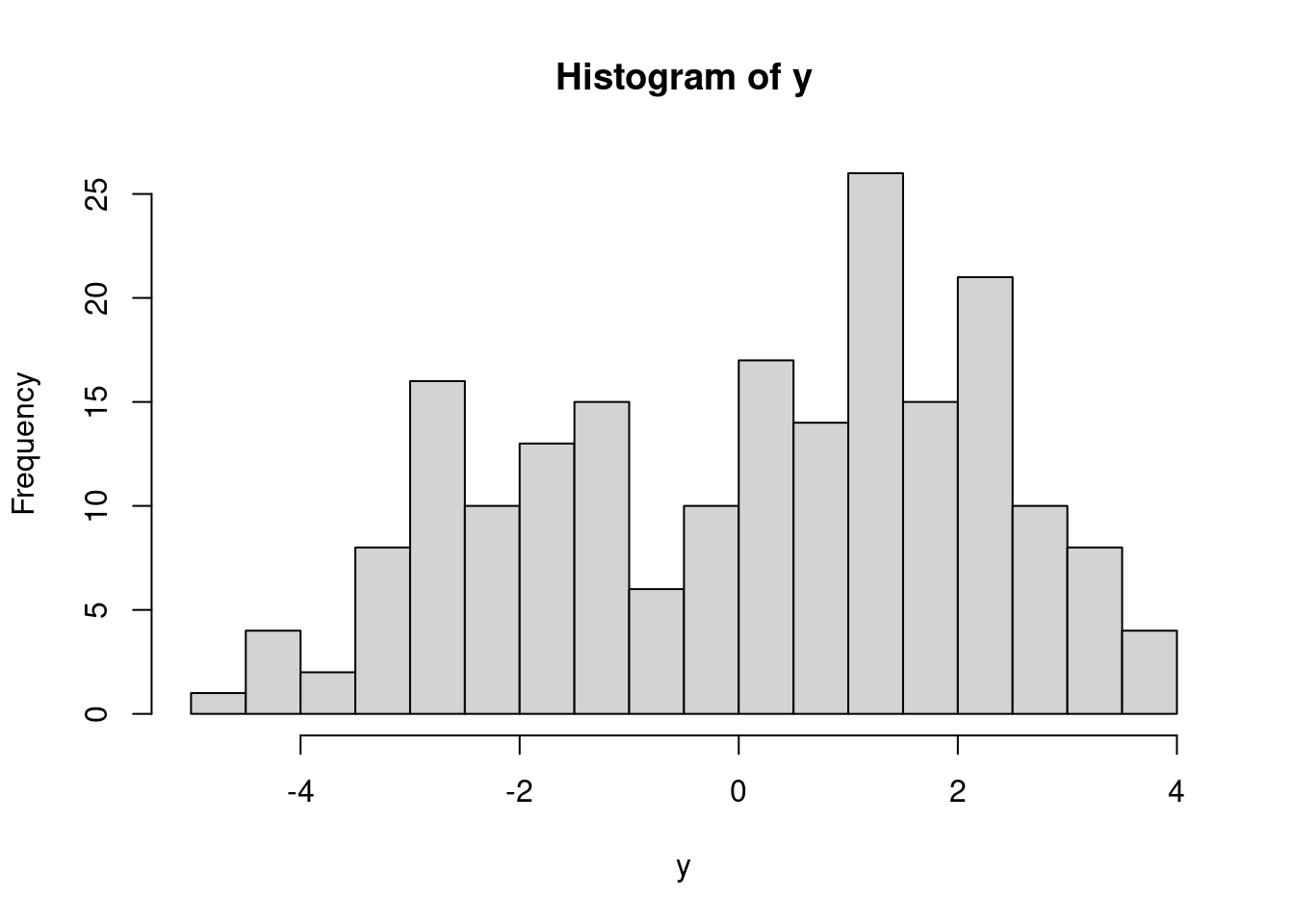
Let's visualize these data.
```{r}
#| label: fig-mixture-data-hist
hist(y, breaks=20)
```
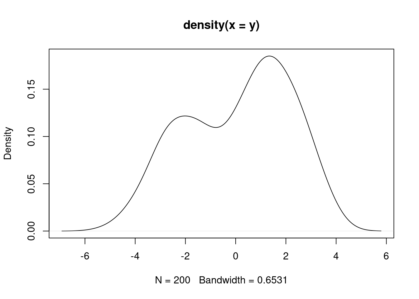
```{r}
#| label: fig-mixture-data-density
plot(density(y))
```
It appears that we have two populations, but we do not know which population each observation belongs to. We can learn this, along with the mixture weights and population-specific parameters with a Bayesian hierarchical model.
We will use a mixture of two normal distributions with variance 1 and different (and unknown) means.
### Model
```{r}
#| label: load-rjags-mixture
library("rjags")
```
```{r}
#| label: mixture-model-string
mod_string = " model {
    for (i in 1:length(y)) {
        y[i] ~ dnorm(mu[z[i]], prec)
      z[i] ~ dcat(omega)
    }

  mu[1] ~ dnorm(-1.0, 1.0/100.0)
    mu[2] ~ dnorm(1.0, 1.0/100.0) T(mu[1],) # ensures mu[1] < mu[2]

    prec ~ dgamma(1.0/2.0, 1.0*1.0/2.0)
  sig = sqrt(1.0/prec)

    omega ~ ddirich(c(1.0, 1.0))
} "

set.seed(11)

data_jags = list(y=y)

params = c("mu", "sig", "omega", "z[1]", "z[31]", "z[49]", "z[6]") # Select some z's to monitor

mod = jags.model(textConnection(mod_string), data=data_jags, n.chains=3)
update(mod, 1e3)

mod_sim = coda.samples(model=mod,
                        variable.names=params,
                        n.iter=5e3)
mod_csim = as.mcmc(do.call(rbind, mod_sim))
```
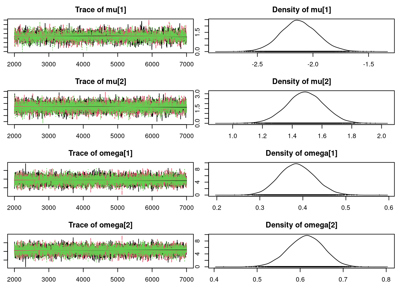
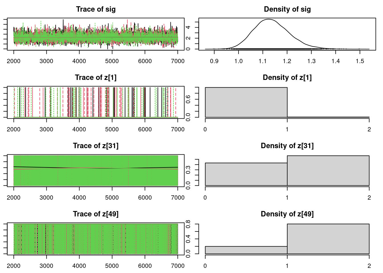
```{r}
#| label: fig-mixture-convergence
## convergence diagnostics
par(mar = c(2.5, 1, 2.5, 1))
plot(mod_sim, ask=TRUE)
```
```{r}
#| label: lst-mixture-convergence-diagnostics
autocorr.diag(mod_sim)
effectiveSize(mod_sim)
```
### Results
```{r}
#| label: lst-mixture-model-summary
summary(mod_sim)
```
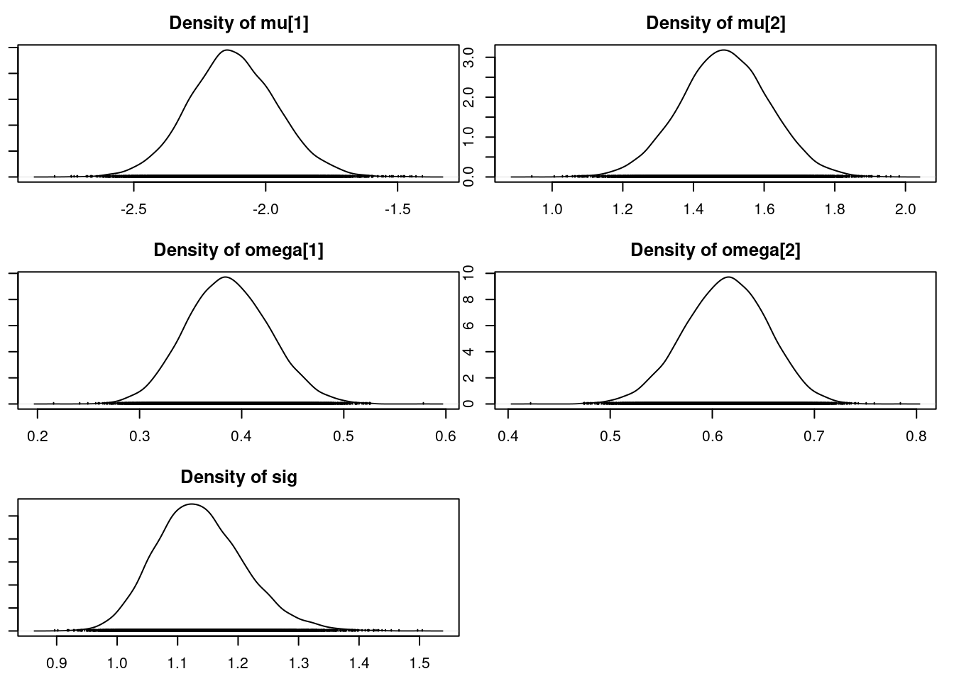
```{r}
#| label: fig-mixture-densities
## for the population parameters and the mixing weights

par(mar = c(2.5, 1, 2.5, 1))
par(mfrow=c(3,2))
densplot(mod_csim[,c("mu[1]", "mu[2]", "omega[1]", "omega[2]", "sig")])
```
```{r}
#| label: fig-mixture-z-densities
## for the z's
par(mfrow=c(2,2))
par(mar = c(2.5, 1, 2.5, 1))
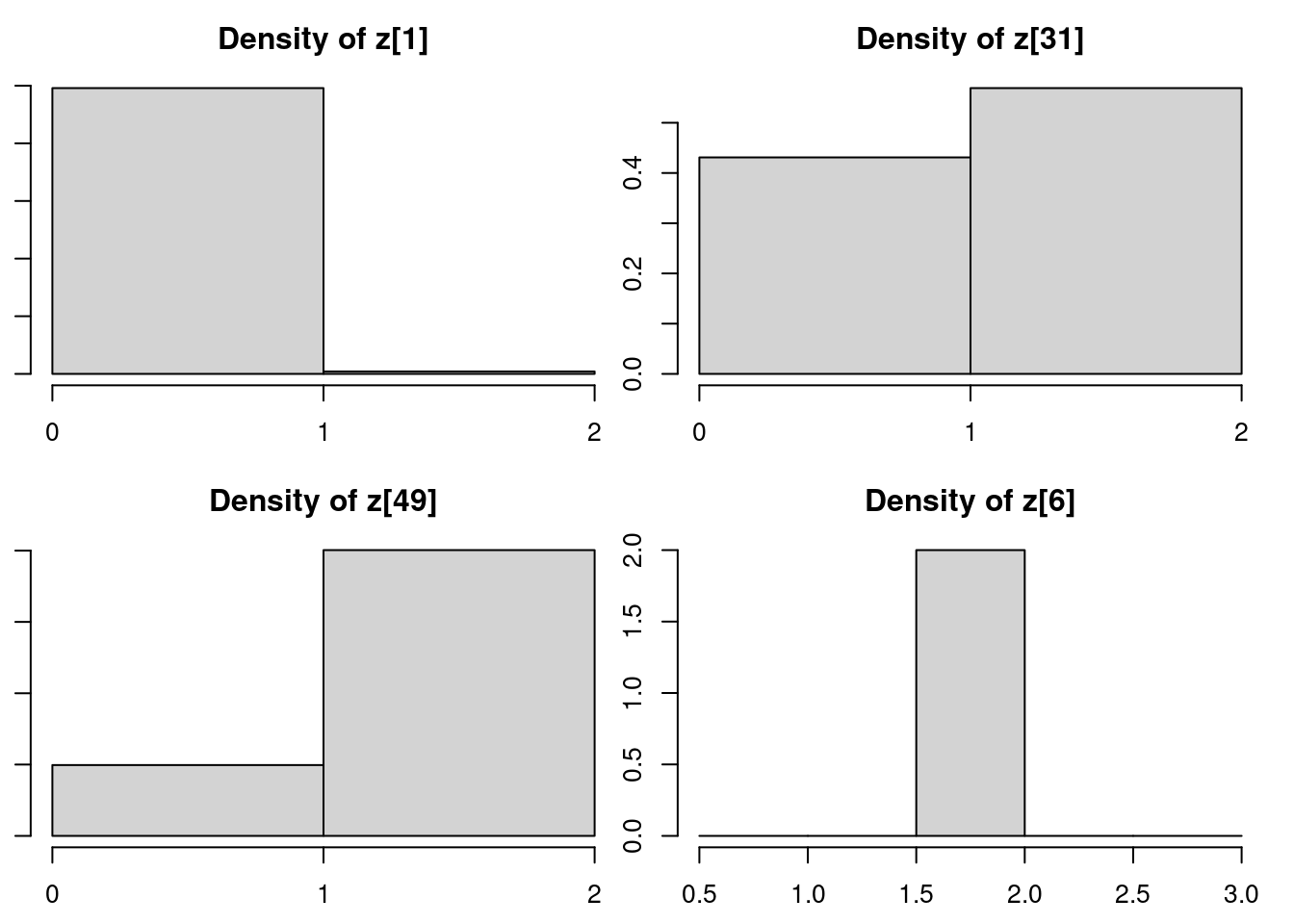
densplot(mod_csim[,c("z[1]", "z[31]", "z[49]", "z[6]")])
```
```{r}
#| label: lst-mixture-z-posterior-probabilities
table(mod_csim[,"z[1]"]) / nrow(mod_csim) ## posterior probabilities for z[1], the membership of y[1]
```
```{r}
#| label: lst-mixture-z-posterior-probabilities-31
table(mod_csim[,"z[31]"]) / nrow(mod_csim) ## posterior probabilities for z[31], the membership of y[31]
```
```{r}
#| label: lst-mixture-z-posterior-probabilities-49
table(mod_csim[,"z[49]"]) / nrow(mod_csim) ## posterior probabilities for z[49], the membership of y[49]
```
```{r}
#| label: lst-mixture-z-posterior-probabilities-6
table(mod_csim[,"z[6]"]) / nrow(mod_csim) ## posterior probabilities for z[6], the membership of y[6]
```
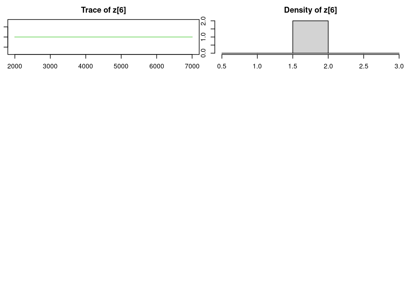
```{r}
#| label: lst-mixture-z-values
y[c(1, 31, 49, 6)]
```
If we look back to the $y$ values associated with these $z$ variables we monitored, we see that $y_1$ is clearly in Population 1's territory, $y_{31}$ is ambiguous, $y_{49}$ is ambiguous but is closer to Population 2's territory, and $y_6$ is clearly in Population 2's territory. The posterior distributions for the $z$ variables closely reflect our assessment.