25.1 Non-Informative Priors
We’ve seen examples of choosing priors that contain a significant amount of information. We’ve also seen some examples of choosing priors where we’re attempting to not put too much information in to keep them vague.
Another approach is referred to as objective Bayesian statistics or inference where we explicitly try to minimize the amount of information that goes into the prior.
This is an attempt to have the data have maximum influence on the posterior
Let’s go back to coin flipping
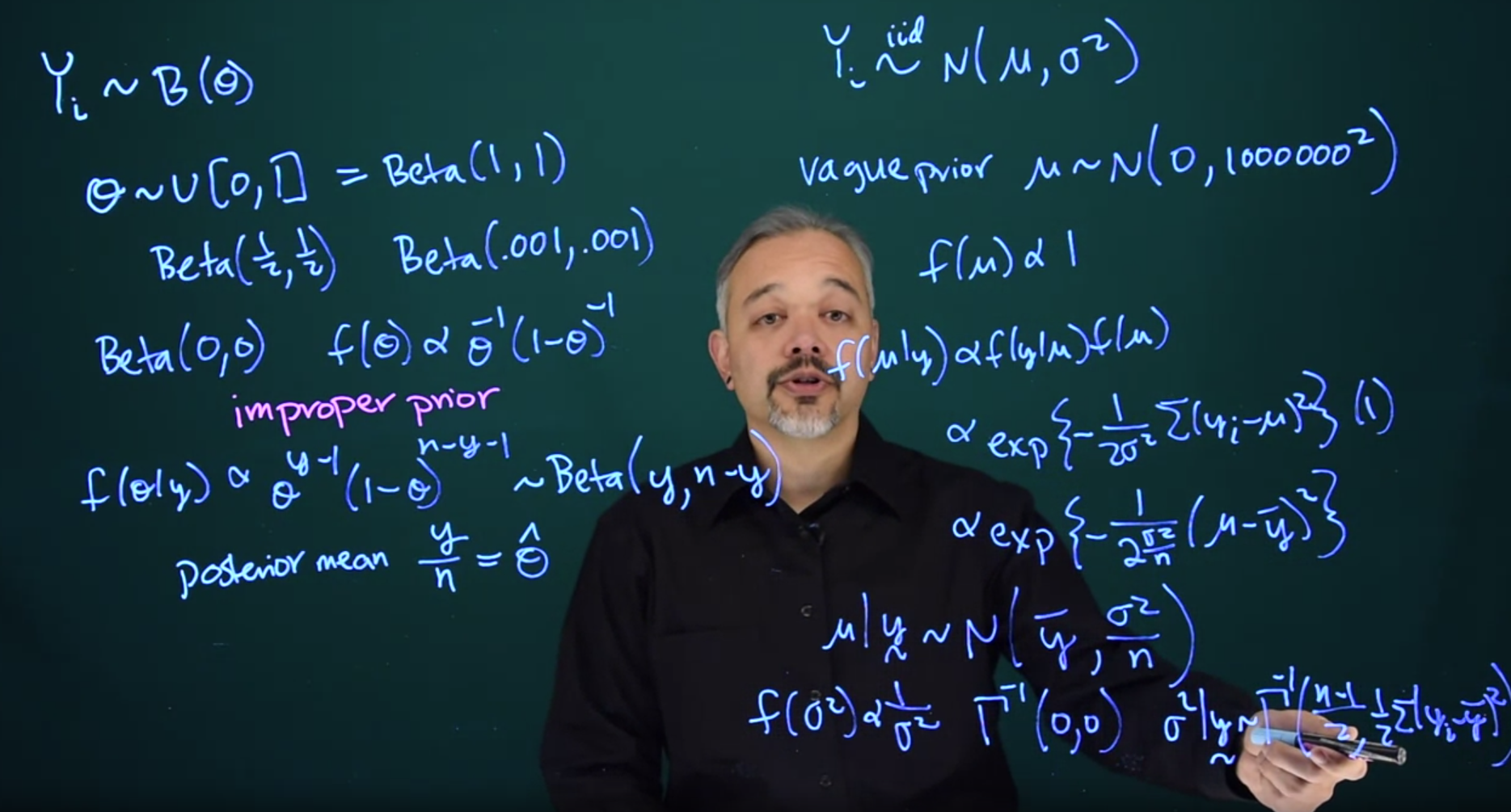
Y_i \sim B(\theta)
How do we minimize our prior information in \theta? One obvious intuitive approach is to say that all values of \theta are equally likely. So we could have a prior for \theta which follows a uniform distribution on the interval [0, 1]
Saying all values of \theta are equally likely seems like it would have no information in it.
Recall however, that a Uniform(0, 1) is the same as Beta(1, 1)
The effective sample size of a beta prior is the sum of its two parameters. So in this case, it has an effective sample size of 2. This is equivalent to data, with one head and one tail already in it.
So this is not a completely non-informative prior.
We could think about a prior that has less information. For example \mathrm{Beta}(\tfrac{1}{2}, \tfrac{1}{2}), this would have half as much information with an effective sample size of one.
We can take this even further. Think about something like \mathrm{Beta}(0.001, 0.001) This would have much less information, with the effective sample size fairly close to zero. In this case, the data would determine the posterior and there would be very little influence from the prior.
25.1.1 Improper priors
Can we go even further? We can think of the limiting case. Let’s think of Beta(0,0), what would that look like?
f(\theta) \propto \theta^{-1}(1-\theta)^{-1}
This is not a proper density. If you integrate this over (0,1), you’ll get an infinite integral, so it’s not a true density in the sense of it not integrating to 1.
There’s no way to normalize it, since it has an infinite integral. This is what we refer to as an improper prior.
It’s improper in the sense that it doesn’t have a proper density. But it’s not necessarily improper in the sense that we can’t use it. If we collect data, we use this prior and as long as we observe one head and one tail, or at least one success and one failure. Then we can get a posterior
f(\theta\mid y) \propto \theta^{y-1}(1-\theta)^{n-y-1} \sim Beta(y, n-y)
With a posterior mean of \frac{y}{n} =\hat{\theta}, which you should recognize as the maximum likelihood estimate. So by using this improper prior, we get a posterior which gives us point estimates exactly the same as the frequentist approach.
But in this case, we can also think of having a full posterior. From this, we can make interval statements, and probability statements, and we can actually find an interval and say that there’s 95\% probability that \theta is in this interval. This is not something you can do under the frequentist approach even though we may get the same exact interval.
25.1.2 Statements about improper priors
Improper priors are okay as long as the posterior itself is proper. There may be some mathematical things that need to be checked and you may need to have certain restrictions on the data. In this case, we needed to make sure that we observed at least one head and one tail to get a proper posterior.
But as long as the posterior is proper, we can go forwards and do Bayesian inference even with an improper prior.
The second point is that for many problems there does exist a prior, typically an improper prior that will lead to the same point estimates as you would get under the frequentist paradigm. So we can get very similar results, results that are fully dependent on the data, under the Bayesian approach.
But in this case, we can also continue to have a posterior and make posterior interval estimates and talk about the posterior probabilities of the parameter.
25.1.3 Normal Case
Another example is thinking about the normal case.
Y_i \stackrel{iid}\sim \mathcal{N}(\mu, \sigma^2) \tag{25.1}
Let’s start off by assuming that \sigma^2 is known and we’ll just focus on the mean \mu.
We can think about a vague prior like before and say that:
\mu \sim N(0, 1000000^2) \tag{25.2}
This would just spread things out across the real line. That would be a fairly non-informative prior covering a lot of possibilities. We can then think about taking the limit, what happens if we let the variance go to \infty. In that case, we’re spreading out this distribution across the entire real number line. We can say that the density is just a constant across the whole real line.
f(\mu) \propto 1
This is an improper prior because if you integrate the real line you get an infinite answer. However, if we go ahead and find the posterior
f(\mu \mid y) \propto f(y \mid \mu) f(\mu) \propto \exp \left (-\frac{1}{2\sigma^2}\sum{(y_i - \mu)^2} \right ) (1)
f(\mu \mid y) \propto \exp(-\frac{1}{2\sigma^2/n}(\mu - \bar{y})^2)
\mu \mid y \sim \mathcal{N}(\bar{y}, \frac{\sigma^2}{n})
This should look just like the maximum likelihood estimate.
25.1.4 Normal with unknown Variance
In the case that \sigma^2 is unknown, the standard non-informative prior is
f(\sigma^2) \propto \frac{1}{\sigma^2}
\sigma^2 \sim \Gamma^{-1}(0,0)
This is an improper prior and it’s uniform on the log scale of \sigma^2.
In this case, we’ll end up with a posterior for \sigma^2
\sigma^2 \mid y \sim \Gamma^{-1}\left (\frac{n-1}{2}, \frac{1}{2}\sum{(y_i - \bar{y})^2}\right)
This should also look reminiscent of the quantities we get as a frequentist. For example, the samples standard deviation
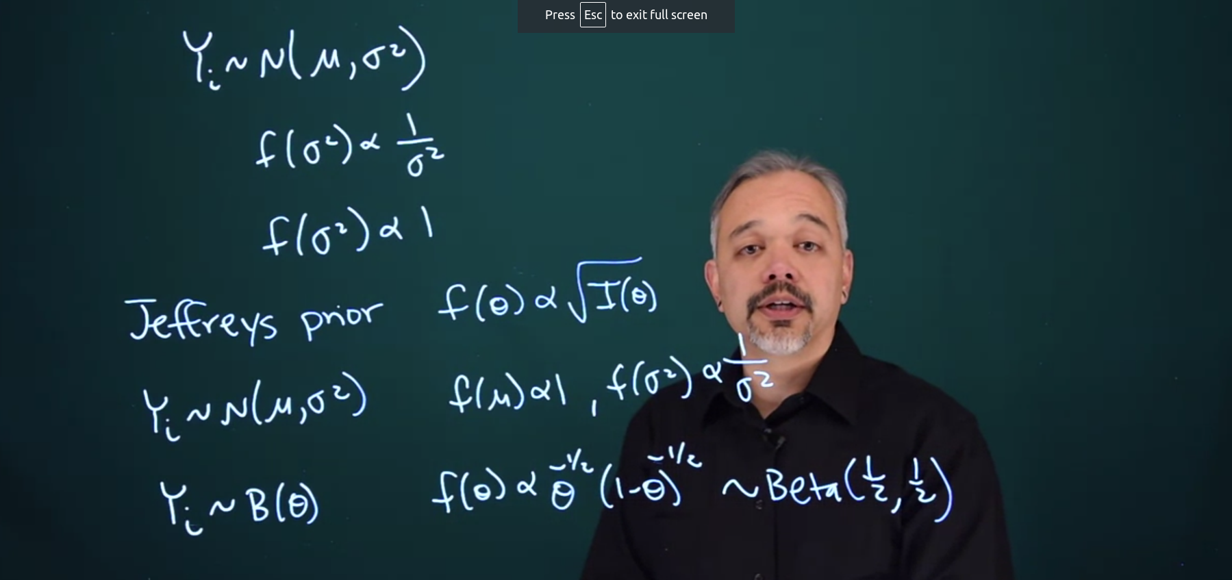
25.2 Jeffrey’s Prior
Choosing a uniform prior depends upon the particular parameterization.
Suppose I used a prior which is uniform on the log scale for \sigma^2
f(\sigma^2) \propto \frac{1}{\sigma^2}
Suppose somebody else decides, that they just want to put a uniform prior on \sigma^2 itself.
f(\sigma^2) \propto 1
These are both uniform on certain scales or certain parameterizations, but they are different priors. So when we compute the posteriors, they will be different as well.
The key thing is that uniform priors are not invariant with respect to transformation. Depending on how you parameterize the problem, you can get different answers by using a uniform prior
One attempt to round this out is to use Jeffreys Prior
Jeffrey’s Prior is defined as the following
f(\theta) \propto \sqrt{\mathcal{I(\theta)}}
Where \mathcal{I}(\theta) is the fisher information of \theta.
In most cases, this will be an improper prior.
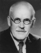
Jeffreys’ Prior is due to Sir Harold Jeffreys (1891-1989) a British geophysicist who who used sophisticated mathematical models to study the Earth and solar system. His hypotheses were uncertain, requiring revision in the face of incoming results, Jeffreys tried to construct a formal theory of scientific reasoning based on Bayesian probability. He made significant contributions to mathematics and statistics. His book, Theory of Probability (Jeffreys 1983), first published in 1939, played an important role in the revival of the objective Bayesian view of probability.
Inductive and Reductive Inference
“The fundamental problem of scientific progress, and a fundamental one of everyday life, is that of learning from experience. Knowledge obtained in this way is partly merely description of what we have already observed, but part consists of making inferences from past experience to predict future experience. This part may be called generalization or induction.”
JEFFREYS’ RULES FOR A THEORY OF INDUCTIVE INFERENCE
- All hypotheses used must be explicitly stated and the conclusions must follow from the hypotheses.
- A theory of induction must be self-consistent; that is, it must not be possible to derive contradictory conclusions from the postulates and any given set of observational data.
- Any rule given must be applicable in practice. A definition is useless unless the thing defined can be recognized in terms of the definition when it occurs. The existence of a thing or the estimate of a quantity must not involve an impossible experiment.
- A theory of induction must provide explicitly for the possibility that inferences made by it may turn out to be wrong.
- A theory of induction must not deny any empirical proposition a priori; any precisely stated empirical proposition must be formally capable of being accepted in the sense of the last rule, given a moderate amount of relevant evidence.
- The number of postulates should be reduced to a minimum. (Occam’s Razor)
- Although we do not regard the human mind as a perfect reasoner, we must accept it as a useful one and the only one available. The theory need not represent actual thought processes in detail but should agree with them in outline.
- In view of the greater complexity of induction, we cannot hope to develop it more thoroughly than deduction. We therefore take it as a rule that an objection carries no weight if an analogous objection invalidates part of generally accepted pure mathematics.
25.2.1 Normal Data
For the example of Normal Data
Y_i \sim N(\mu, \sigma^2)
f(\mu) \propto 1
f(\sigma^2) \propto \frac{1}{\sigma^2}
Where \mu is uniform and \sigma^2 is uniform on the log scale.
This prior will then be transformation invariant. We will end up putting the same information into the prior even if we use a different parameterization for the Normal.
25.2.2 Binomial
Y_i \sim B(\theta)
f(\theta) \propto \theta^{-\frac{1}{2}}(1-\theta)^{-\frac{1}{2}} \sim \mathrm{Beta}(\frac{1}{2},\frac{1}{2})
This is a rare example of where the Jeffrey’s prior turns out to be a proper prior.
You’ll note that this prior actually does have some information in it. It’s equivalent to an effective sample size of one data point. However, this information will be the same, not depending on the parameterization we use.
In this case, we have \theta as a probability, but another alternative which is sometimes used is when we model things on a logistics scale.
By using the Jeffreys prior, we’ll maintain the exact same information.
25.2.3 Closing information about priors
Other possible approaches to objective Bayesian inference include priors such as reference priors and maximum entropy priors.
A related concept to this is called empirical Bayesian analysis. The idea in empirical Bayes is that you use the data to help inform your prior; such as by using the mean of the data to set the mean of the prior distribution. This approach often leads to reasonable point estimates in your posterior. However, it’s sort of cheating since you’re using your data twice and as a result may lead to improper uncertainty estimates.
25.3 Fisher Information
The Fisher information (for one parameter) is defined as
\mathcal{I}(\theta) = E\left[\left(\frac{d}{d\theta}log{(f(X \mid \theta))}\right)^2\right]
Where the expectation is taken with respect to X which has PDF f(X \mid \theta). This quantity is useful in obtaining estimators for \theta with good properties, such as low variance. It is also the basis for Jeffrey’s prior.
Use of the Jeffreys prior violates the strong version of the likelihood principle. Which proposes that, given a statistical model, all the evidence in a sample relevant to model parameters is contained in the likelihood function. When using the Jeffreys prior, inferences about \theta depend not just on the probability of the observed data as a function of \theta, but also on the universe of all possible experimental outcomes, as determined by the experimental design, because the Fisher information is computed from an expectation over the chosen universe. Accordingly, the Jeffreys prior, and hence the inferences made using it, may be different for two experiments involving the same \theta parameter even when the likelihood functions for the two experiments are the same a violation of the strong likelihood principle.
Example 25.1 (Jeffreys prior) Let
X \mid \theta \sim N(\theta, 1)
Then we have
f(x \mid \theta) = \frac{1}{\sqrt{2\pi}}\exp[-\frac{1}{2}(x-\theta)^2]
\log{(f(x \mid \theta))} = -\frac{1}{2}\log{(2\pi)}-\frac{1}{2}(x-\theta)^2
\left ( \frac{d}{d\theta}log{(f(x \mid \theta))} \right )^2 = (x-\theta)^2
and so
\mathcal{I}(\theta) = \mathbb{E}[(X - \theta)^2] = \mathbb{V}ar[X] = 1
25.4 Sensitivity analysis of priors
The general approach to using priors in models is to start with some justification for a prior, run the analysis, then come up with competing priors and reexamine the conclusions under the alternative priors. The results of the final model and the analysis of the sensitivity of the analysis to the choice of prior are written up as a package.
For a discussion of steps and methods to use in a sensitivity analysis, see: (Gelman et al. 2013, page: 38) which discusses two approaches:
Many times we choose priors out of convenience. How to judge when assumptions of convenience can be made safely is a central task of Bayesian sensitivity analysis.
- Analysis using different conjugate prior distributions.
Starting with a uniform prior
More informative priors are tested and the 95% posterior CI is compared against the posterior mean and the prior mean.
A table of prior mean, prior effective sample size , posterior mean and posterior 95 CI is created for the results
We are interested primarily to see how well the the posterior CI can excludes the prior mean even for priors with large effective sample size.
- Analysis using a non-conjugate prior distribution follows the same approach but uses non conjugate prior. The comparisons described in 1. can be carried out using sampling.
(Gelman et al. 2013, pages: 141)