31.1 Components of a Bayesian Model 🎥
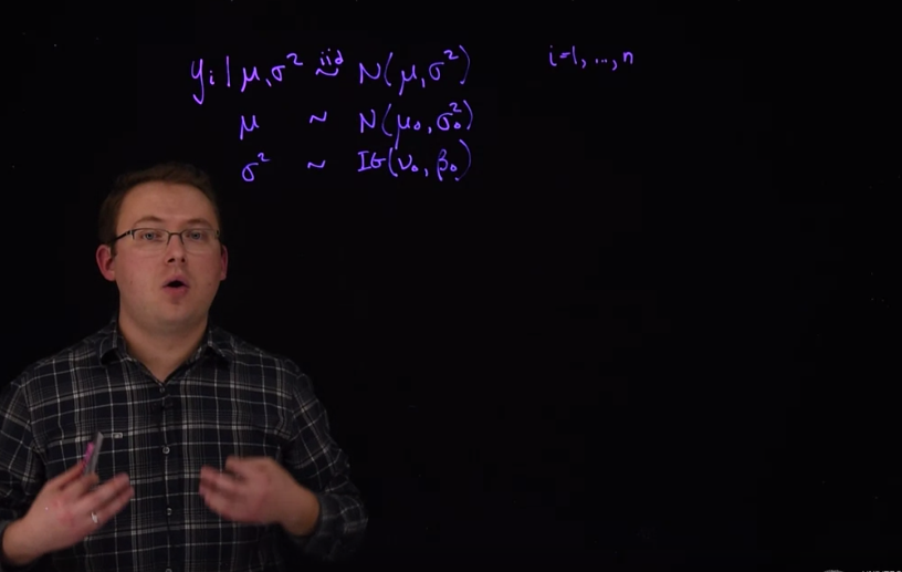
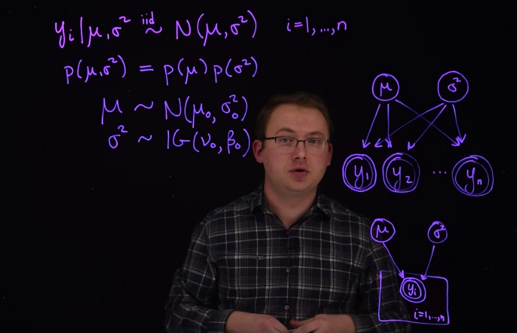
\begin{aligned} y_i \mid \mu,\sigma &\stackrel{iid}{\sim} \mathcal{N}(\mu,\sigma^2) \\ \mu &\sim \mathcal{N}(\mu_0,\sigma_0^2) \\ \sigma^2 &\sim \mathcal{IG}(\alpha_0,\beta_0) \end{aligned} \tag{31.1}
In lesson one, we defined a statistical model as a mathematical structure used to imitate or approximate the data generating process. It incorporates uncertainty and variability using the theory of probability. A model could be very simple, involving only one variable.
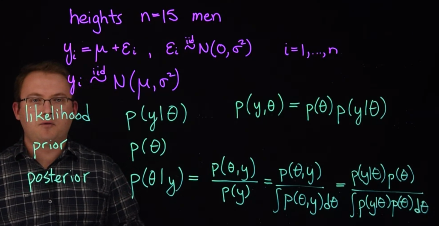
Example 31.1 (heights of men) Suppose our data consists of the heights of N=15 adult men. Clearly it would be very expensive or even impossible to collect the genetic information that fully explains the variability in these men’s heights. We only have the height measurements available to us. To account for the variability, we might assume that the men’s heights follow a normal distribution.
heights of men
So we could write the model like this: y_i= \mu + \varepsilon_i
- where:
- y_i will represent the height for person i.
- i will be our index.
- \mu is a constant that represents the mean for all men.
- \varepsilon_i, the individual error term for individual i.
We are also going to assume that these uncertainties \varepsilon_i are drawn independently from an the same normal distribution. We can make this more precise if we specify that the \varepsilon_i a drawn from a normal distribution with mean zero and variance \sigma^2.
\varepsilon_i \stackrel{iid}\sim \mathcal{N}(0,\sigma^2) \quad i\in 1 \dots N
- where:
- i equal to 1 up to N which will be 15 in our case.
Equivalently1 we could rewrite this model expressing the variability for the y_i directly as:
y_i \stackrel{iid}\sim \mathcal{N}(\mu,\sigma^2) \quad i \in 1 \dots N
What we did is substitute Normal RV of \varepsilon then push in the mean \mu into the RV. Which is shown in the example below. So each y_i is drawn independently from identically distributed RV with a Normal distribution parameterized with mean \mu and variance \sigma^2. This specifies a probability distribution and a model for the data.
Noteheights of men
\begin{aligned} y_i&= \mu+\varepsilon_i, \\ \varepsilon_i &\stackrel{iid}\sim \mathcal{N}(0,\sigma^2) \end{aligned} another way to write this if we know the values of \mu and \sigma:
\begin{aligned} y_i &\stackrel{iid}\sim \mathcal{N}(\mu,\sigma^2) \end{aligned}
It also suggests how we might generate more fake data that behaves similarly to our original data set.
A model can be as simple as the one right here or as complicated and sophisticated as we need to capture the behavior of the data. So far, this model is the same for Frequentists and Bayesians.
As you may recall from the previous course, the frequentist approach to fitting this model would be to consider \mu and \sigma to be fixed but unknown constants, and then we would estimate them. To calculate our uncertainty in those estimates a frequentist approach would consider how much the estimates of \mu and \sigma might change if we were to repeat the sampling process and obtain another sample of 15 men, over, and over.
The Bayesian approach, which we will follow in this class, treats our uncertainty in \mu and \sigma^2 using probabilities directly. We will model them as random variables with their own probability distributions. These are often called priors, and they complete a Bayesian model.
uncertainty \to random variables
In the rest of this segment, we’re going to review the three key components of Bayesian models, that were used extensively in the previous course. These three primary components of Bayesian models which we often work with are:
- \mathbb{P}r(y\mid \theta) the likelihood of the data,
- \mathbb{P}r(\theta) the prior distribution for the parameters,
- \mathbb{P}r(\theta \mid y) the posterior distribution for the parameters given the data
\mathbb{P}r(y\mid \theta)\ \text{(likelihood)}
The likelihood is the probabilistic model for the data. It describes how, given the unknown parameters, the data might be generated. We’re going to call unknown parameter theta right here. Also, in this expression, you might recognize this from the previous class, as describing a probability distribution.
The likelihood
\mathbb{P}r(\theta)\ \text{(prior)}
The prior, the next step, is the probability distribution that characterizes our uncertainty with the parameter theta. We’re going to write it as \mathbb{P}r(\theta). It’s not the same distribution as this one. We’re just using this notation \mathbb{P}r to represent the probability distribution of \theta.
The prior
By specifying a likelihood and a prior. We get have a joint probability model for both the knowns, i.e. the data, and the unknowns, i.e. the parameters \theta.
joint probability distribution
\mathbb{P}r(y,\theta) = \underbrace{\mathbb{P}r(\theta)}_{prior} \cdot \underbrace{\mathbb{P}r(y \mid \theta)}_{likelihood} \qquad \text{(joint probability)}
We can see this by using the chain rule of probability. If we wanted the joint distribution of both the data and the parameters theta. Using the chain rule of probability, we could start with the distribution of \theta and multiply that by the probability of y \mid \theta. That gives us an expression for the joint distribution. However if we’re going to make inferences about data and we already know the values of y, we don’t need the joint distribution, what we need is the posterior distribution.
posterior distribution
\mathbb{P}r(\theta \mid y)\ \text{(posterior)}
The posterior distribution is the distribution of \mathbb{P}r(\theta \mid y), i.e. \theta given y. We can obtain this expression using the laws of conditional probability and specifically using Bayes’ theorem.
\begin{aligned} \mathbb{P}r(\theta \mid y) &= \frac{\mathbb{P}r(\theta,y)}{\mathbb{P}r(y)} \\ &= \frac{\mathbb{P}r(\theta,y)}{\int \mathbb{P}r(\theta,y)} \\ &= \frac{\mathbb{P}r(y \mid \theta)\ \mathbb{P}r(\theta)}{\int \mathbb{P}r(y \mid \theta)\ \mathbb{P}r(\theta)\ d\theta} \end{aligned}
We start with the definition of conditional probability (1). The conditional distribution, \mathbb{P}r(\theta \mid y) is the ratio of the joint distribution of \theta and y, i.e. \mathbb{P}r(\theta,y); with the marginal distribution of y, \mathbb{P}r(y).
We start with the joint distribution like we have on top, and we integrate out or marginalize over the values of theta (2)
How do we get the marginal distribution of y?
To make this look like the Bayes theorem that we’re familiar with the joint distribution can be rewritten as the product of the prior and the likelihood. We start with the likelihood, because that’s how we usually write Bayes’ theorem. We have the same thing in the denominator here. But we’re going to integrate over the values of theta. These integrals are replaced by summations if we know that \theta is a discrete random variable. The marginal distribution is another important piece which we may use when we more advanced Bayesian modeling.
The posterior distribution is our primary tool for achieving the statistical modeling objectives from lesson one.
NoteAnatomy of a posterior probability
\begin{aligned} &\mathbb{P}r(y\mid \theta) && (likelihood) \\ & \mathbb{P}r(\theta) && (prior) \\ \mathbb{P}r(y,\theta) &= \mathbb{P}r(\theta)\mathbb{P}r(y|\theta) &&(joint\ distribution) \\ \mathbb{P}r(\theta \mid y) &= \frac{\mathbb{P}r(\theta,y)}{\mathbb{P}r(y)} && (conditional\ probability) \\ &= \frac{\mathbb{P}r(\theta,y)}{\int \mathbb{P}r(\theta,y)} \\ &= \frac{\mathbb{P}r(y \mid \theta)\ \mathbb{P}r(\theta)}{\int \mathbb{P}r(y \mid \theta)\ \mathbb{P}r(\theta)\ d\theta} \\ \end{aligned} \tag{31.2}
Whereas non-Bayesian approaches consider a probability model for the data only, the hallmark characteristic of Bayesian models is that they specify a joint probability distribution for both data and parameters. How does the Bayesian paradigm leverage this additional assumption?
31.2 Model Specification 🎥
Before fitting any model we first need to specify all of its components.
31.2.1 Hierarchical representation
One convenient way to do this is to write down the hierarchical form of the model. By hierarchy, we mean that the model is specified in steps or in layers. We usually start with the model for the data directly, or the likelihood. Let’s write, again, the model from the previous lesson.
We had the height for person i, given our parameters \mu and \sigma^2, so conditional on those parameters, y_i came from a normal distribution that was independent and identically distributed, where the normal distribution has mean \mu and variance \sigma^2, and we’re doing this for individuals 1 up to N, which was 15 in this example.
y_i \mid \mu,\sigma^2 \stackrel{iid}\sim N(\mu,\sigma^2) \qquad \forall \ i \in 1,\dots,15
The next level that we need is the prior distribution from \mu and \sigma^2. For now we’re going to say that they’re independent priors. So that our prior from \mu and \sigma^2 is going to be able to factor Into the product of two independent priors.
\mathbb{P}r(\mu,\sigma^2)~=~\mathbb{P}r(\mu)\mathbb{P}r(\sigma^2)\qquad (independence)
We can assume independents in the prior and still get dependents in the posterior distribution.
In the previous course we learned that the conjugate prior for \mu, if we know the value of \sigma^2, is a normal distribution, and that the conjugate prior for \sigma^2 when \mu is known is the Inverse Gamma distribution.
Let’s suppose that our prior distribution for \mu is a normal distribution where mean will be \mu_0.
\mu \sim \mathcal{N}(\mu_0,\sigma^2_0)
This is just some number that you’re going to fill in here when you decide what the prior should be. Mean \mu_0, and less say \sigma^2_0 would be the variance of that prior.
The prior for \sigma^2 will be Inverse Gamma
\sigma^2 \sim \mathcal{IG}(\nu_0,\beta_0)
- which has two parameters:
- a shape parameter, \nu_0, and
- a scale parameter, \beta_0.
We need to choose values for these hyper-parameters here. But we do now have a complete Bayesian model.
We now introduce some new ideas that were not presented in the previous course.
NoteHierarchical representation
By hierarchy, we mean that the model is specified in steps or in layers.
- start with the model for the data, or the likelihood.
- write the priors
- add hyper-priors for the parameters of the priors.
More details can be seen on this wikipedia article and on this one
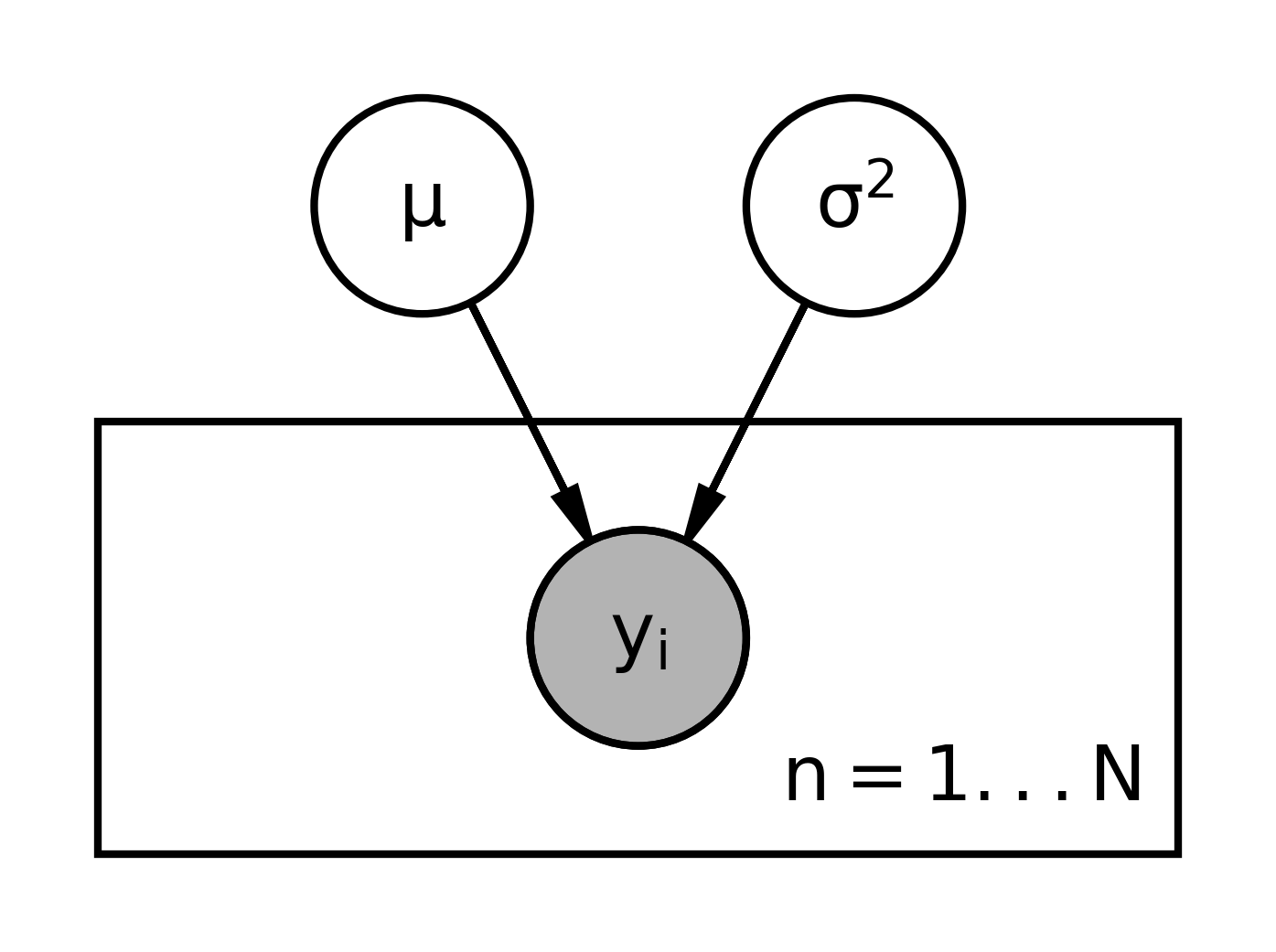
31.2.2 Graphical representation
Another useful way to write out this model Is using what’s called a graphical representation. To write a graphical representation, we’re going to do the reverse order, we’ll start with the priors and finish with the likelihood.
In the graphical representation we draw what are called nodes so this would be a node for mu. The circle means that the this is a random variable that has its own distribution. So \mu with its prior will be represented with that. And then we also have \sigma^2. The next part of a graphical model is showing the dependence on other variables. Once we have the parameters, we can generate the data.
For example we have y_1, \dots y_n. These are also random variables, so we’ll create these as nodes. And I’m going to double up the circle here to indicate that these nodes are observed, you see them in the data. So we’ll do this for all of the y_i here. And to indicate the dependence of the distributions of the y_i on \mu and \sigma^2, we’re going to draw arrows. So \mu influences the distribution of y for each one of these y_i. The same is true for sigma squared, the distribution of each y depends on the distribution of \sigma^2. Again, these nodes right here, that are double-circled, mean that they’ve been observed. If they’re shaded, which is the usual case, that also means that they’re observed. The arrows indicate the dependence between the random variables and their distributions.
Notice that in this hierarchical representation, I wrote the dependence of the distributions also. We can simplify the graphical model by writing exchangeable random variables and I’ll define exchangeable later.
We’re going to write this using a representative of the y_i here on what’s called the plate. So I’m going to re draw this hierarchical structure, we have \mu and \sigma^2. And we don’t want to have to write all of these notes again. So I’m going to indicate that there are n of them, and I’m just going to draw one representative, y_i. And they depend on \mu and \sigma^2. To write a model like this, we must assume that the y_i are exchangeable. That means that the distribution for the y_i does not change if we were to switch the index label like the i on the y there. So, if for some reason, we knew that one of the y_i was different from the other y_i in its distribution, and if we also know which one it is, then we would need to write a separate node for it and not use a plate like we have here.
NoteGraphical representation
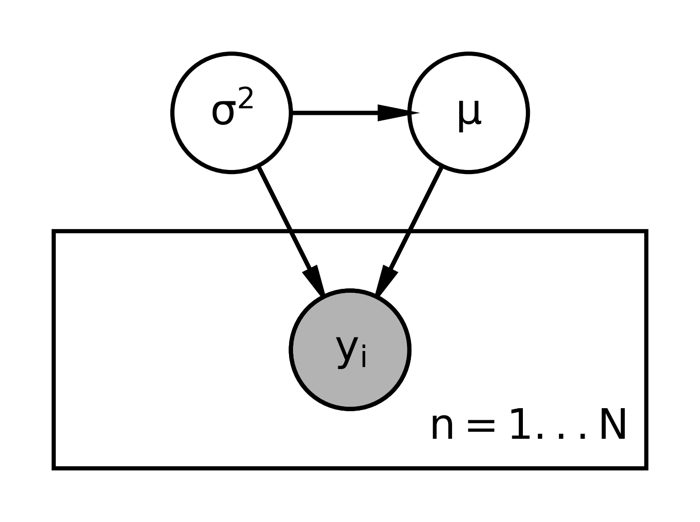
In the graphical representation we start at the top by drawing:
- circle nodes for the hyperparameters.
- arrows indicating that they determine the
- nodes for the priors.
- nodes for the RVs (doubled circles)
- plates (rectangles) indicating RVs that are exchangeable. We add an index to the corner of the plate to indicate the amount of replicated RVs
More details can be seen on this wikipedia article
Both the hierarchical and graphical representations show how you could hypothetically simulate data from this model. You start with the variables that don’t have any dependence on any other variables. You would simulate those, and then given those draws, you would simulate from the distributions for these other variables further down the chain.
This is also how you might simulate from a prior predictive distribution.
31.3 Posterior derivation 🎥
So far, we’ve only drawn the model with two levels. But in reality, there’s nothing that will stop us from diving deeper into the rabbit hole and adding more layers.
For example, instead of fixing the values for the hyperparameters in the previous segment recall those hyperparameters were the \mu_0, the \sigma_0, the \nu_0 and the \beta_0, we could either specify fixed numeric values for those, or we could try to infer them from the data and model them using additional prior distributions for those variables to make this a hierarchical model.
A good reason to construct the model hierarchically is if the data generating process is organized in levels so that groups of observations generated at a certain level are more naturally grouped e.g there is greater similarity within groups than between groups together for each subsequent levels. We will examine these types of hierarchical models in depth later in the course. Another simple example of a hierarchical model is one you saw already in the previous course c.f. Section 23.2
Back to our model:
- At the top level are the observation: y_i \mid \mu,\sigma^2. This is just like the model from the previous lesson, where the observations were from independent and identically distributed normal RV with a mean \mu and a variance, \sigma^2.
- At the next level we diverge, instead of having independent priors for \mu and \sigma^2, we’re going to have the prior for \mu depend on the value of \sigma^2. That is given \sigma^2, \mu follows a normal distribution with mean \mu_0, just some hyperparameter that you’re going to chose. And the variance of this prior will be \sigma^2, this parameter, divided by \omega_0. Another hyperparameter that will scale it.
\begin{aligned} y_i \mid \mu,\sigma^2 &\stackrel{iid}{\sim} \mathcal{N}(\mu,\sigma^2) \\ \mu \mid \sigma^2 &\sim \mathcal{N}(\mu_0,\frac{\sigma^2}{\omega_0}) \\ \sigma^2 \mid &\sim \mathcal{IG}(\nu_0,\beta_0) \end{aligned} \tag{31.3}
- where:
- \mu_0 is the mean of the prior for \mu,
- \omega_0 is a scaling factor for the variance of the prior for \mu,
- \nu_0 and \beta_0 are the shape and scale parameters of the inverse gamma prior for \sigma^2.
We now have a joint distribution of y \mid \mu and \mu \mid \sigma^2 To complete this model we need to provide a prior for \sigma^2.
- We’ll just use the standard Inverse-Gamma with the same hyperparameters as last time.
The graphical representation for this model looks like this:
NoteGraphical representation
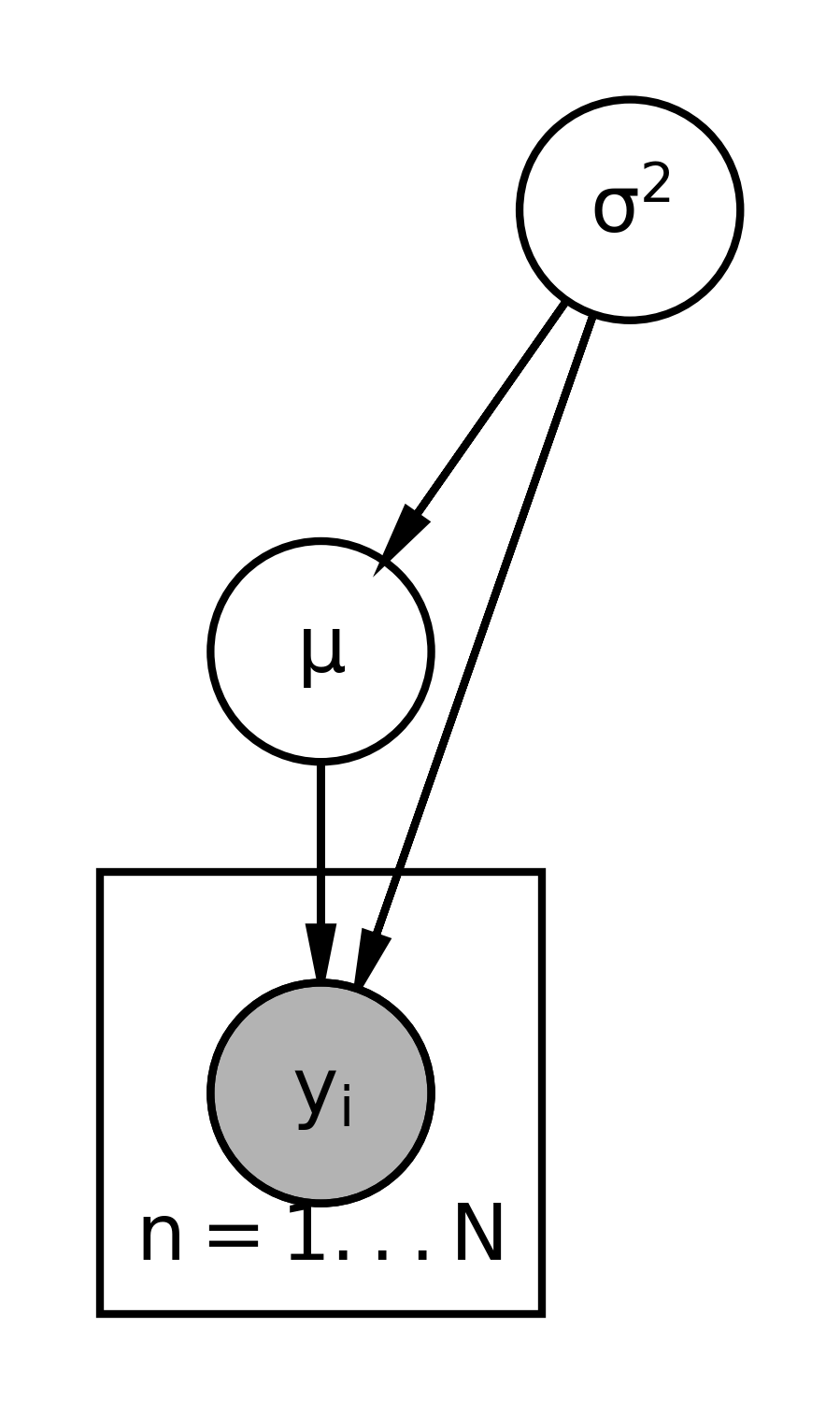
- We start with the variables that don’t depend on anything else.
- That would be \sigma^2 and move down the chain.
- The next variable is \mu, which depends on \sigma^2.
- Then we have the y_i dependent on both, We use a double or filled circle because the y_i’s are observed, their data, and we’re going to assume that they’re exchangeable.
- We place the y_i’s on a plate for i \in 1 \dots N.
- The distribution of y_i depends on both \mu and \sigma^2, so we’ll draw curves connecting those pieces there.
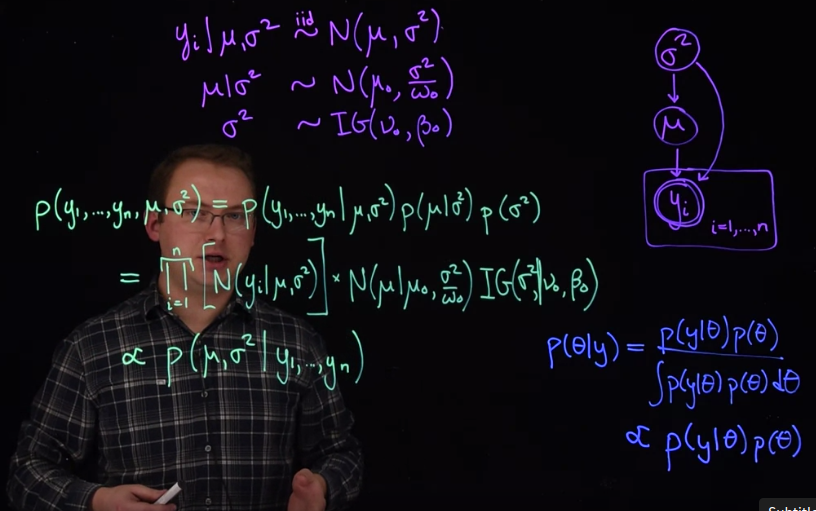
\begin{aligned} p(\mu \mid y_i \dots y_n) &\propto \prod_{i=1}^{n} \left[\frac{1}{\sqrt{2 \pi \sigma^2}} \exp\left(-\frac{(y_i - \mu)^2}{2 \sigma^2}\right)\right] \cdot \frac{1}{\pi(1 + \mu^2)} \\ &\propto \exp \left[\left(-\frac{(y_i - \mu)^2}{2 \sigma^2}\right) \right ] \cdot \frac{1}{(1 + \mu^2)} \\ &\propto \frac{ \exp \left[ n (\bar{y} - \frac{\mu^2}2{}) \right] }{1 + \mu^2} \end{aligned}
To simulate hypothetical data from this model, we would have to first draw from the distribution of the prior for \sigma^2. Then the distribution for mu which depends on \sigma^2. And once we’ve drawn both of these, then we can draw random draws from the y_i, which of course depends on both of those. With multiple levels, this is an example of a hierarchical model. Once we have a model specification, we can write out what the full posterior distribution for all the parameters given the data looks like. Remember that the numerator in Bayes’ theorem is the joint distribution of all random quantities, all the nodes in this graphical representation over here from all of the layers. So for this model that we have right here, we have a joint distribution that’ll look like this. We’re going to write the joint distribution of everything y_1:n, \mu and \sigma^2, using the chain rule of probability, we’re going to multiply all of the distributions in the hierarchy together. So let’s start with the likelihood piece. And we’ll multiply that by the next layer, the distribution of mu, given \sigma^2. And finally, with the prior for sigma squared. So what do these expressions right here look like?
The likelihood in this level because they’re all independent will be a product of normal densities. So we’re going to multiply the normal density for each y_i, given those parameters. This, again, is shorthand right here for the density of a normal distribution. So that represents this piece right here. The conditional prior of \mu given sigma squared is also a normal. So we’re going to multiply this by a normal distribution of \mu, where its parameters are \mu naught and sigma squared over omega naught. And finally, we have the prior for sigma squared. We’ll multiply by the density of an inverse gamma for \sigma^2 given the hyper parameters \mu naught, sorry, that is given, the hyper parameters \mu naught and and beta naught. What we have right here is the joint distribution of everything. It is the numerator in Bayes theorem. Let’s remind ourselves really fast what Bayes theorem looks like again. We have that the posterior distribution of the parameter given the data is equal to the likelihood, Times the prior. Over the same thing again. So this gives us in the numerator the joint distribution of everything which is what we’ve written right here.
In Bayes theorem, the numerator and the denominator are the exact same expression accept that we integrate or marginalize over all of the parameters.
Because the denominator is a function of the y’s only, which are known values, the denominator is just a constant number. So we can actually write the posterior distribution as being proportional to, this symbol right here represents proportional to. The joint distribution of the data and parameters, or the likelihood times the prior. The poster distribution is proportional to the joint distribution, or everything we have right here. In other words, what we have already written for this particular model is proportional to the posterior distribution of \mu and \sigma^2, given all of the data. The only thing missing in this expression right here is just some constant number that causes the expression to integrate to 1. If we can recognize this expression as being proportional to a common distribution, then our work is done, and we know what our posterior distribution is. This was the case for all models in the previous course. However, if we do not use conjugate priors or if the models are more complicated, then the posterior distribution will not have a standard form that we can recognize. We’re going to explore a couple of examples of this issue in the next segment.
31.4 Non-conjugate models 🎥
We’ll first look at an example of a one parameter model that is not conjugate.
31.4.0.1 Company Personnel
Suppose we have values that represent the percentage change in total personnel from last year to this year for, we’ll say, ten companies. These companies come from a particular industry. We’re going to assume for now, that these are independent measurements from a normal distribution with a known variance equal to one, but an unknown mean.
So we’ll say the percentage change in the total personnel for company I, given the unknown mean \mu will be distributed normally with mean \mu, and we’re just going to use variance 1.
In this case, the unknown mean could represent growth for this particular industry.
It’s the average of the growth of all the different companies. The small variance between the companies and percentage growth might be appropriate if the industry is stable.
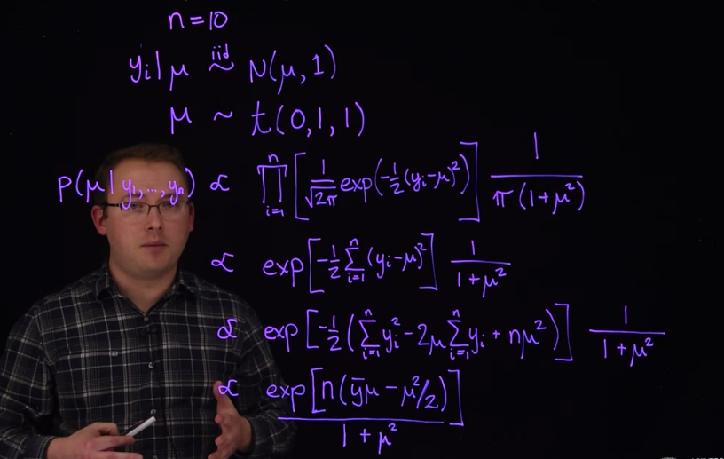
We know that the conjugate prior for \mu in this location would be a normal distribution.
But suppose we decide that our prior believes about \mu are better reflected using a standard t distribution with one degree of freedom. So we could write that as the prior for \mu is a t distribution with a location parameter 0. That’s where the center of the distribution is. A scale parameter of 1 to make it the standard t-distribution similar to a standard normal, and 1 degree of freedom.
This particular prior distribution has heavier tails than the conjugate and normal distribution, which can more easily accommodate the possibility of extreme values for \mu. It is centered on zero so, that apriori, there is a 50% chance that the growth is positive and a 50% chance that the growth is negative.
Recall that the posterior distribution of \mu is proportional to the likelihood times the prior. Let’s write the expression for that in this model. That is the posterior distribution for \mu given the data y_1 \dots y_n is going to be proportional to the likelihood.
It is a product from i equals 1 to n, in this case that’s 10.
Densities from a normal distribution.
Let’s write the density from this particular normal distribution.
Is 1 \over \sqrt{2 \pi}.
E to the negative one-half.
y_i - \mu^2, this is the normal density for each individual y_i and we multiplied it for likelihood.
The density for this t prior looks like this.
It’s 1 over pi times 1 plus \mu squared.
This is the likelihood times the prior.
If we do a little algebra here, first of all, we’re doing this up to proportionality.
So, constants being multiplied by this expression are not important.
The \sqrt{2 \pi}^n, is just a constant number, and \pi creates a constant number. So we will drop them in our next step.
So this is now proportional too, we’re removing this piece and now we’re going to use properties of exponents.
The product of exponents is the sum of the exponentiated pieces.
So we have the exponent of negative one-half times the sum from i equals 1 to n, of Yi minus \mu squared.
And then we’re dropping the pie over here, so times 1 plus \mu squared.
We’re going to do a few more steps of algebra here to get a nicer expression for this piece.
But we’re going to skip ahead to that.
We’ve now added these last two expressions.
To arrive at this expression here for the posterior, or what’s proportional to the posterior distribution.
This expression right here is almost proportional to a normal distribution except we have this 1 plus \mu squared term in the denominator.
We know the posterior distribution up to a constant but we don’t recognize its form as a standard distribution.
That we can integrate or simulate from, so we’ll have to do something else.
Let’s move on to our second example. For a two parameter example, we’re going to return to the case where we have a normal likelihood.
And we’re now going to estimate \mu and \sigma^2, because they’re both unknown.
Recall that if \sigma^2 were known, the conjugate prior from \mu would be a normal distribution.
And if \mu were known, the conjugate prior we could choose for \sigma^2 would be an inverse gamma.
We saw earlier that if you include \sigma^2 in the prior for \mu, and use the hierarchical model that we presented earlier, that model would be conjugate and have a closed form solution. However, in the more general case that we have right here, the posterior distribution does not appear as a distribution that we can simulate or integrate.
Challenging posterior distributions like these ones and most others that we’ll encounter in this course kept Bayesian methods from entering the main stream of statistics for many years. Since only the simplest problems were tractable. However, computational methods invented by physicists in the 1950’s, and implemented by statisticians decades later, revolutionized the field. We now do have the ability to simulate from the posterior distributions from this lesson, as well as for many other more complicated models.
via the linearity of the normal distribution in the mean↩︎