---
title : 'MCMC for Mixture Models - M4L1'
subtitle : 'Bayesian Statistics: Mixture Models'
categories:
- Bayesian Statistics
keywords:
- Mixture Models
- MCMC
- Markov Chain Monte Carlo
- notes
---
\index{mixture!MCMC algorithm}
Markov chain Monte Carlo (MCMC) algorithm are typically used to perform Bayesian inference in complex models.
In MCMC algorithms we repeatedly sample from the full conditional distributions of each block of parameters given fixed values for the rest.
After an appropriate burn-in period, they generate samples that are dependent but identically distributed according to the posterior distribution of interest.
## Markov Chain Monte Carlo algorithms part 1 ::video_camera::
{#fig-s_01 .column-margin width="53mm" group="slides"}
{#fig-s_02 .column-margin width="53mm" group="slides"}
::: {.callout-tip}
## Notation
1. under-tildes signify a vector or collection.
2. $\{i:c_i=l\}$ mean the sum over the indices for a specific component $k$. We are regrouping the rows by their components
3. The double product mean we are iterating over the data rows times their likelihoods. (as usual)
4. The indicator in the exponent mean we are only taking one term per row which is picked using the component for which the latent indicator is true.
:::
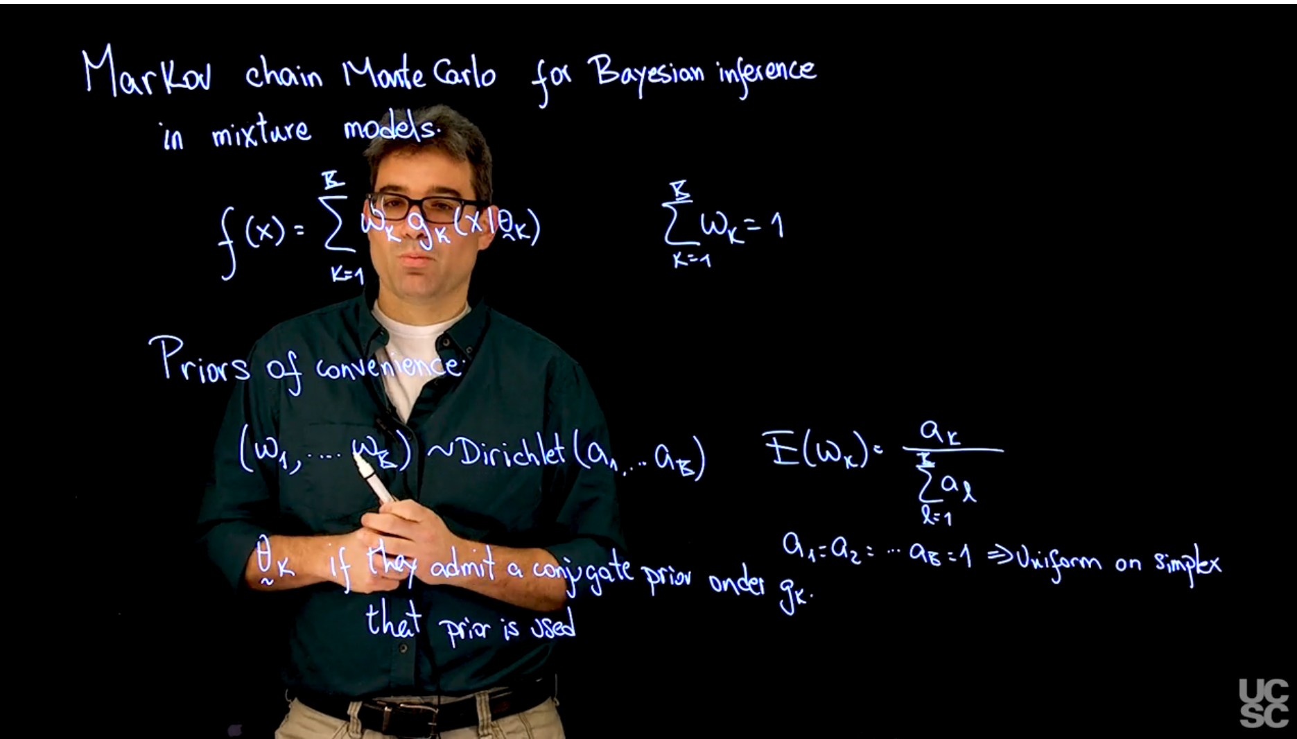
The model takes the form :
$$
f(x\mid \theta) = \sum_{k=1}^K w_k g(x \mid \theta_k)
$$ {#eq-mixture-model}
The model is defined by the parameters $\theta = (\theta_1, \ldots, \theta_K)$ and the weights $w = (w_1, \ldots, w_K)$.
In the Bayesian setting we also need priors for the weights and the parameters of each components.
$$
(w_1, \ldots, w_K) \sim \textrm{Dirichlet}(\alpha_1, \ldots, \alpha_K) \qquad \mathbb{E}[w_k] = \frac{\alpha_k}{\sum_{k=1}^K \alpha_k}
$$ {#eq-parameter-prior}
also if we use $a_1 = a_2 = ... a_k=1$ we end up with a uniform prior on the simplex.
- $\tilde{\theta}_k$ if they admit a conjugate prior, we can use the conjugate prior for the parameters of the component $k$. Even though it won't be conjugate for the whole model, it will be conjugate for the component $k$, at least given the sampling scheme outlined in [@eq-complete-data-likelihood-sampling-scheme].
$$
\mathbb{P}r(w) = \frac{\Gamma(\sum_{k=1}^K \alpha_k)}{\prod_{k=1}^K \Gamma(\alpha_k)} \prod_{k=1}^K w_k^{\alpha_k - 1} \qquad \sum_{k=1}^K w_k = 1
$$ {#eq-dirichlet-prior}
To develop a MCMC algorithm for mixture models we will use the hierarchical representation of the likelihood,
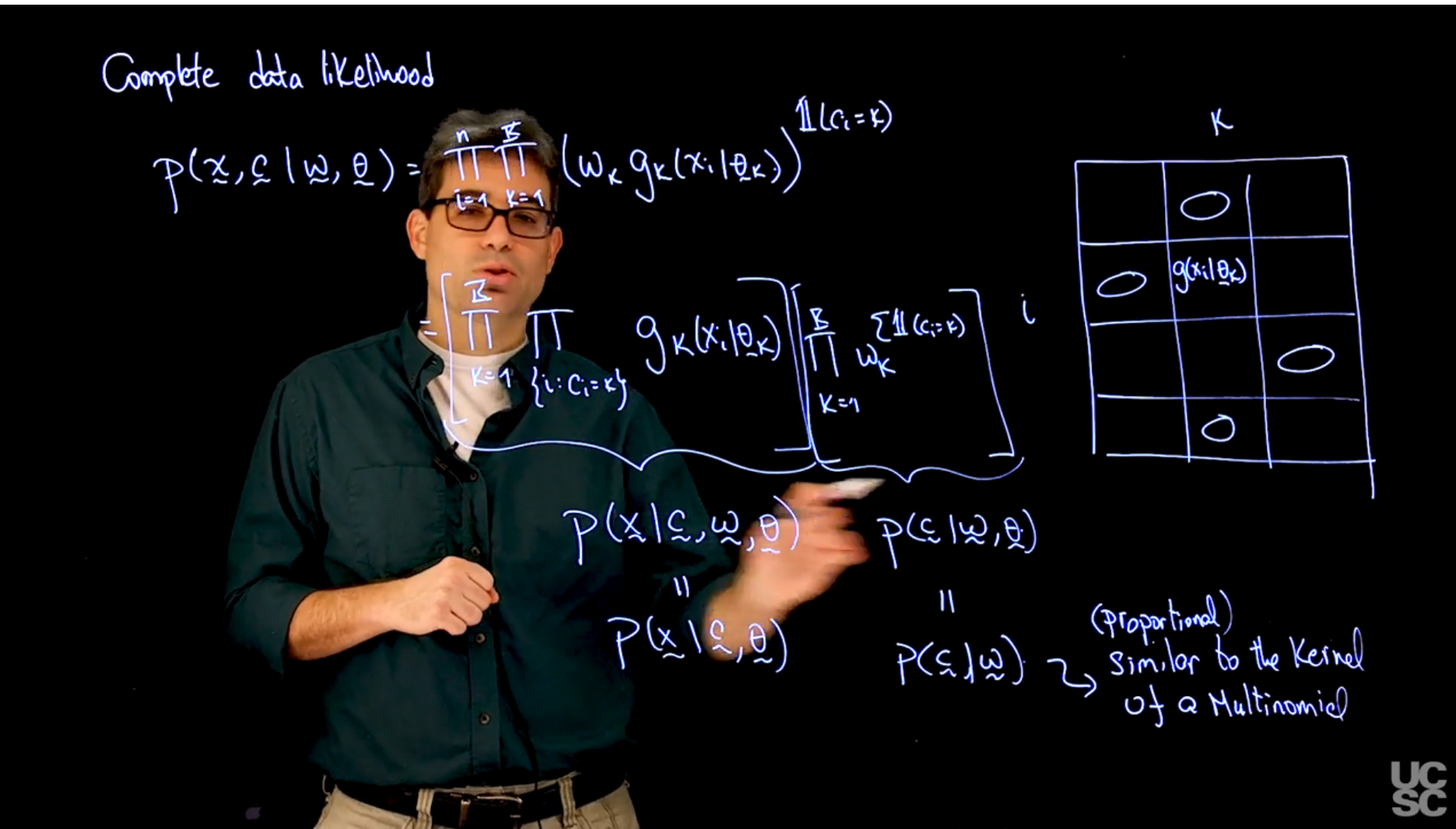
Complete data likelihood:
$$
\begin{aligned}
\mathbb{P}r(\mathbf{x}, \mathbf{c}, \mid \mathbf{\omega}, \mathbf{\theta}) &= \prod_{i=1}^n \prod_{k=1}^K (\omega_k\ g_k(x_i \mid \theta_k))^{\mathbb{1}(c_i = k)} &
\\& = \left[\prod_{k=1}^K \prod_{\{i:c=k\}}^n g_k(x_i \mid \theta_k)\right] && \left [\prod_{k=1}^n \omega_{k}^{\sum \mathbb{1}(c_i = k)}\right ]
\\& = \mathbb{P}r(\mathbf{x} \mid \mathbf{c}, \mathbf{\omega}, \mathbf{\theta}) && \mathbb{P}r(\mathbf{c} \mid \mathbf{\omega}, \mathbf{\theta})
\\& = \mathbb{P}r(\mathbf{x} \mid \mathbf{c}, \mathbf{\theta}) && \mathbb{P}r(\mathbf{c} \mid \mathbf{\omega})
\end{aligned}
$$ {#eq-complete-data-likelihood-sampling-scheme}
The logic in this derivation is that we can rewrite the complete data likelihood as a product of two terms where we separate the weight from the other parameters.
::: {.callout-warning collapse="true"}
## Unclear !? {.unnumbered .unlisted}
I'm not sure this is 100% correct, we seem to be trying to write out the fact that each component is conditionally independent given the weights and the component parameters.
This step from the first line to the second line is based on regrouping the terms in the product based on component $k$.
Another issue now that I've made an effort to clarify the notation is that the selection of the term in the product is based on picking the kernel from just one component.
But it seems that we don't know how to infer which component the data point belongs to.
:::
In the third line we reinterpreting :
- the left product in line 2 as a product of the likelihoods of the data if we know given their component, weights and parameters.
- the right product in line 2 as the distribution of the indicators given the weights and parameters.
In the last line we remove $\omega$ on from the left term based on independence. And we remove $\theta$ from the right term based on independence.
<!-- TODO: extract transcript to external file and summarize -->
::: {.callout-note collapse="true"}
## Video transcript {.unnumbered .unlisted}
[In previous lectures, we discussed the expectation maximization algorithm for fitting mixture models. In this lecture, we are going to discuss Markov Chain Monte Carlo for Bayesian inference in mixture models.]{.mark}
[We're going to move from frequentist inference which we were interested only on finding the point estimate for the parameters in the model to a situation in which we are going to try to explore a full posterior distribution for those parameters.]{.mark}
[Recall that the mixture model we are working with is going to take the form or the density of that mixture model.]{.mark}
It is going to take the form of f of x is the sum over k components of weight multiplied by the components in the mixture.
Those components are indexed by this parameter theta k, and we may have components that are all belong to the same family or that they belong to different families.
If we are going to do Bayesian inference for this model, we need to compliment this density that is going to give us the likelihood with priors on the unknown parameters.
In particular, we're going to need priors for the weights, and we are going to need priors for the data suitcase. What is typically done in these situations is to use a priors of convenience.
Where are those priors of convenience?
[Well, first for the weights remember that we have a constraint that the sum of the weights needs to be equal to one.]{.mark}
[Obviously each one of them individually needs to be between zero and one. So a natural prior for that type of parameters is a Dirichlet prior and that is precisely what we are going to use.]{.mark}
So we're going to assume that the prior for the vector that includes all these weights just follows a Dirichlet distribution, with parameters a1 all the way to $a_k$.
Just as a quick reminder they expected value of each one of these parameters individually is just given by the corresponding a divided by the sum of the a's.
[So in other words, the values of the a's just constrains a prior that is the relative size of the different weights. ]{.mark}
In particular if you make them all the same, then you are saying that a prior you believe that all the weights are the same.
We also know that as a special case if you make $a_1=a_2= \ldots = a_k$ and in particular equal to one then we just have the Uniform distribution on the simplex.
Which is actually one of the typical choices used for the hyperparameters when fearing mixture models.
Now, this is our priori of convenience for the omegas and we will see that in addition to having a very nice interpretation it will also allow us to do computation in a very straight forward manner.
Now, the other set of priors that we need is the priors for the data case.
What is typically done here is that if they admit a conjugate prior under gk then that prior is used.
[The reason for that is that even though for the full mixture this conjugate prior on the $g_k1$ conjugate for the full model it will be conditionally conjugate under our sampling scheme that we will derive in a minute.]{.mark}
So it will make computation for the parameters theta k much simpler if we can find that conjugate prior under theta k.
After we have set up priors for the model the next thing that we need to do before deriving our Gibbs sampler is to write down the complete data likelihood in a slightly more convenient way.
If you remember the complete data likelihood that we used extensively for deriving the EM Algorithm has the form of the distribution of the data in all those indicators CSU either just tells you which component you belong to conditional on the weight, and all the Thetas is just going to take the form of a double product.
So the product over the observations followed by the product over the components of omega sub k g sub k of x sub y given Theta k raised to the indicator function of ci equals to k.
In other words, rather than write the complete sum that we had before, we replaced that completes sum by a product where each one of the terms is now raised to this indicator function that just depends on whether the component was generated, the observation was generated by the k component in the mixture.
This complete data likelihood that we use extensively can now be written in a couple of different ways, and one that is going to be particularly helpful for us involves breaking this expression into two pieces, one that has to do with their omega's, and one that has to do with g's.
So let me start with a piece that starts with the g's.
The way in which I'm going to do it is first I'm going to reverse the order of this products.
So I am going to consider first the product over the components.
Next I'm going to consider the product over the observations.
But before I write exploration explicitly, let me interpret this expression up here a little bit.
So what we're doing here with this double product or one way to think about what we're doing with a double product is to think about computing a bunch of terms that are in here in particular in this piece, that can be positioned onto a matrix where one dimension corresponds to the index i, and the second dimension corresponds to the index k.
The entries of this matrix are just g of x i given theta k.
So different combinations of i and different combinations of k gives you the values that you are going to put into this matrix.
Now, what is this important?
Because if you think about what they indicator or function up here is doing is it's telling you well you need to compute the whole matrix but you're actually not going to use the full matrix, you are just going to pick a few elements of it, and in particular you are going to pick one element in each row according to what the value of ci case.
So for example, if the first observation belongs to the second component you'd be picking this value, second observation the first component you will pick this value, third observation with third component here and so on.
So the values of the ci can be interpreted as giving you a way to select elements in this matrix, and in particular one per row.
[So another way to write the product over all the observations is used to think about grouping rows together according to which column is being selected. In particular, for example, we could put all the observations that have the first column being selected together, then all the observations that have the second column being selected together and so on.]{.mark}
One way to write that mathematically is to say that we're going to do a product over the i's but grouped together according to the value of k.
Then we can get rid of the indicator and the numerator and write this as g sub k, xi given theta sub k.
So this is one piece of this expression up here or one way to rewrite this expression up here or one piece of it that involves the g-subcase.
Of course we have a second piece that involves the omegas, that second piece that involves the omegas we can write as the product.
Again, I'm going to consider the product over the case first.
Then for a given k, omega k is exactly the same argument for all of them.
So I can just write omega k and the product of omega k to the indicators just becomes omega k raised to the sum of the indicators.
Well, once I have written the expression in this way, I can essentially think about this piece as being the distribution of the observations if I knew the indicators, the omegas, and the thetas.
It so happens that this expression in particular doesn't depend on the omegas.
So for this model this is the same as p of x given c and the theta.
In this expression here you can interpret as the distribution of the c's given the omegas and the theta's.
Again, in the particular structure of this model this happens to just depend on the weights omega.
So we know that the product of these two quantities is just by the total law of probability the expression that we wanted in the beginning that is the distribution of the Theta and indicators together.
So this particular form for the distribution is going to be particularly useful in terms of deriving the posterior distribution that we need for the Gibbs sampler.
One last observation that I want to make that will be useful in the future is that if you think about what is the form of this piece down here the distribution or the Indicators even the weights, what you have is a form that resembles the kernel of multinomial distribution.
So this is similar to the kernel of a multinomial.
In particular, it's not only similar but it's proportional to it.
So it will be particularly useful in terms of deriving the algorithm using the fact that this looks like a multinomial distribution.
:::
## Markov Chain Monte Carlo algorithms part 2 ::video_camera::
{#fig-s_03 .column-margin width="53mm" group="slides"}
{#fig-s_04 .column-margin width="53mm" group="slides"}
{#fig-s_05 .column-margin width="53mm" group="slides"}
Now that we have a structure for the likelihood function that we and the prior distributions for all of our parameters, we can can derive the posterior distribution for our model.
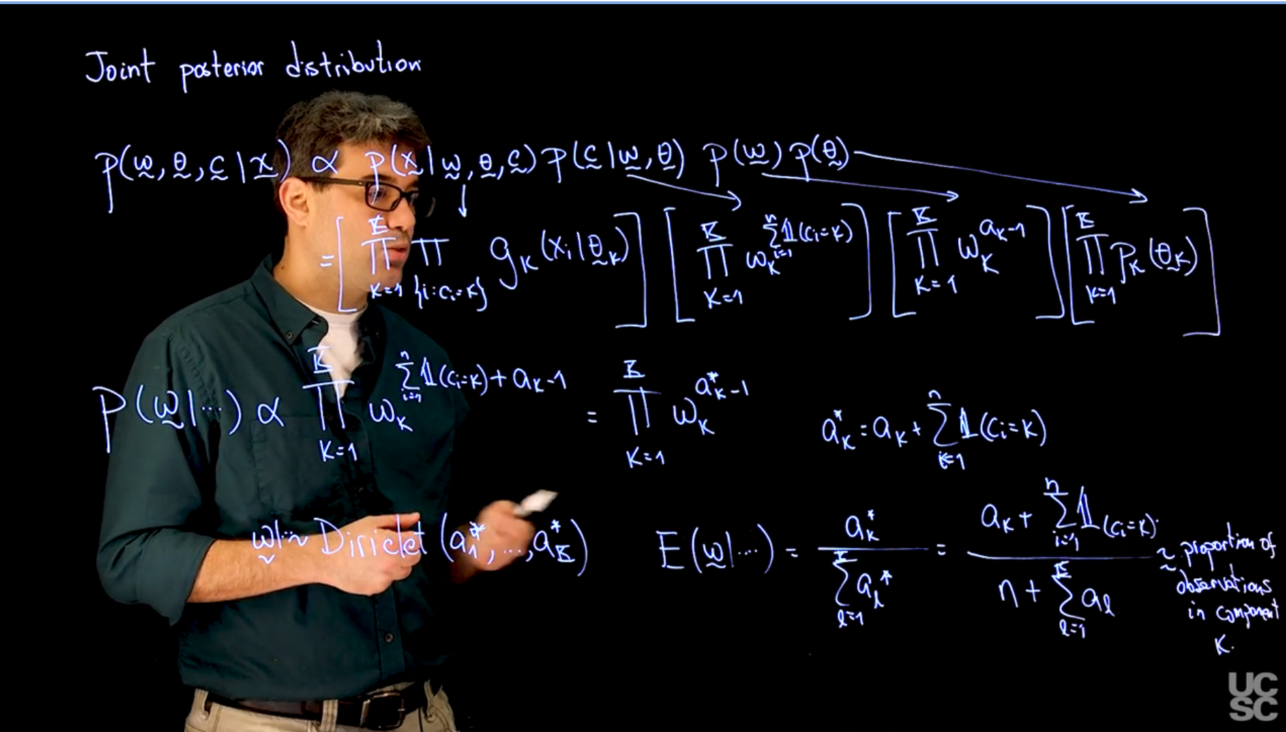
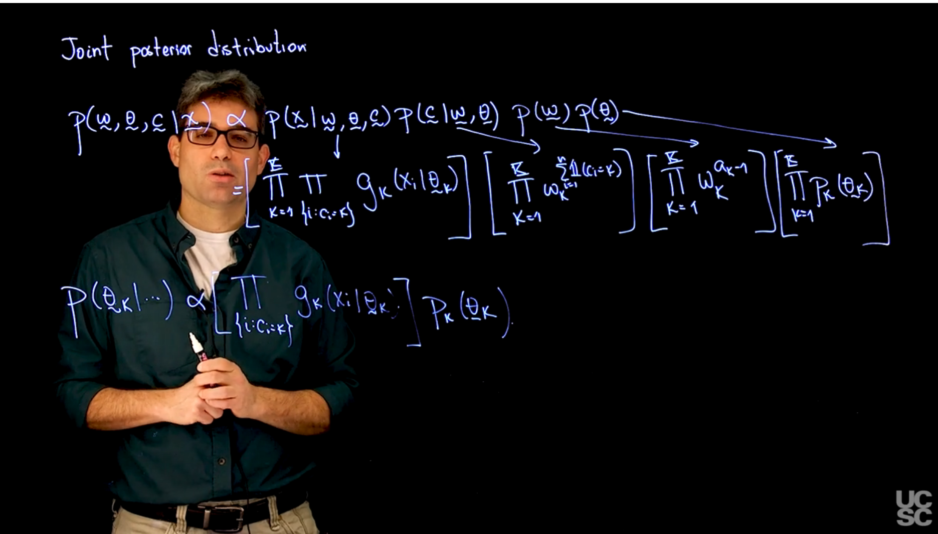
So we want to write down the joint posterior distribution.
In that joint posterior distribution includes, the weights and the parameters of the components, but it also involves the vector of indicators C, that we have introduced to simplify the structure of the likelihood, and by definition, this quantity is proportional to the distribution of the data, given all the parameters, multiplied by the distribution of the missing data parameters, given Omega and Theta, multiplied by the prior distribution on the parameters, multiplied by the prior distribution on the base.
$$
\mathbb{P}r(c, \theta, \omega \mid x) \propto \left \{ \prod_{i=1}^n \mathbb{P}r(x | c, \theta, \omega) \right \} \left \{ \prod_{i=1}^n\prod_{k=1}^K \mathbb{P}r(c \mid \omega, \theta) \right \}\ \mathbb{P}r(\omega)\ \mathbb{P}r(\theta)
$$ {#eq-posterior-distribution}
Each of the full conditional distributions can be derived from this joint posterior by retaining the terms that involve the parameter of interest, and recognizing the product of the selected terms as the kernel of a known family of distributions.
<!-- TODO: extract transcript to external file and summarize -->
::: {.callout-note collapse="true"}
## Video transcript {.unnumbered .unlisted}
[Now that we have a clear structure for the likelihood function that we will be using and we have prior distributions for all of our parameters, we can proceed to derive the posterior distribution that we will be working with.]{.mark}
We want to write down the joint posterior distribution.
In that joint posterior distribution includes, of course, the weights and the parameters of the components, but it also involves the vector of indicators $C$, that we have introduced to simplify the structure of the likelihood, and by definition, this quantity is proportional to the distribution of the data, given all the parameters, multiplied by the distribution of the missing data parameters, given $\omega$ and $\theta$, multiplied by the prior distribution on the parameters, multiplied by the prior distribution on the base.
So this is the general expression, the general form, for that posterior distribution.
Now, we have already seen what the form of the different terms is.
In particular, this joint distribution of the data can be written as a double product.
First-order components, and then over the groups of observations that belong to each one of those components of $g_k$ $x_i$, given $\theta_k$.
So that is the first piece that we're interested in.
The second piece, we have already seen also how to write it down.
This is going to be the product from k equals one, to capital k of $\omega_k$.
Some of these indicators of $c_i$ is equal to k from one to n. This is our second piece.
Then we discussed using a Dirichlet distribution for this. So ignoring some proportionality constants, this becomes the product from k equals one to capital k of $\omega_k$ raised to the $a_k - 1$.
That's this piece.
Then finally, we're going to have another product.
So typically, we use independent priors for each one of the data case.
As I said, we'll typically try to pick them so that they are conjugate to this kernel, $g_k()$, but for now, I'm going to write it in general form by writing this as $p_k(\theta_k)$, and that's what the last term in the expression is. So we have written down a full expression for this.
Now, it should be more or less clear how we need to proceed.
So we need full conditionals for all the parameters in the model.
In particular, we are going to need a full conditional for $\omega$, given all the other parameters, we're going to need a full conditional for each one of the $c_i$'s given the rest of the parameters, and we're going to need a full conditional for each one of the data cases, given the rest of the parameters.
So to derive these full conditionals, what we will do is we will pick particular pieces from this expressions to retain and to construct this
particular four conditionals.
Let's proceed now to derive each one of the four conditionals that we need to derive a Gibbs sampler or a Markov Chain Monte Carlo algorithm for this problem.
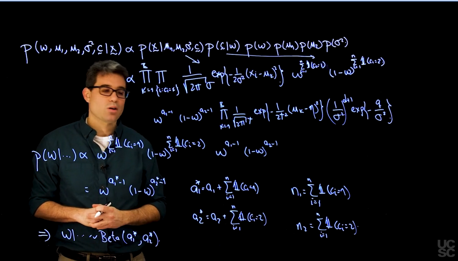
Let's just start with the full posterior distribution for the weights, and please note that we're going to work with all the weights as a block, so we're going to try to sample them all together, and rather than looking at each one of them at a time. o this full conditional distribution is made up of the terms in this full posterior distribution that involves $\omega_k$, and if you look at this expression carefully, you will see that this piece doesn't depend on $\omega_k$ anyway, and that this piece doesn't depend on any of the $\omega_k$ either, so it's just this two pieces in the middle that we need to consider.
Furthermore, the two pieces are very similar, so both in both products over K of the weight raised to some power, so we can actually combine the two expressions together and just write them as the product from one to capital k of $\omega_k$ raised to the sum of these indicator functions, plus a_k minus 1. This looks exactly like
the prior that we used, except that now, we have updated parameters.
So I could write this as the product of $\omega_k$ raised to the $a_k$, call them stars, minus one, where a_k a star, is just the original $a_k$ plus the sum from one to n of the indicators of $c_i$ equals to k.
[So just doing this little change, makes it very clear that the form of the posterior is exactly the same form as the prior.]{.mark}
[In other words, this a conditionally conjugate prior for our problem, and that just means that $\omega$ is going to be distributed as a Dirichlet, given all the other parameters, but with this updated parameters, a_1 star all the way to a_k star, and this is very interesting because essentially, a posteriori, we know that the expected value of $\omega$ given all the other parameters, so this is the expected value of the full conditional. This is not expected value of the marginal posterior, but this is the expected value of the full conditional]{.mark}
that is going to be a_k star divided by the sum from L equals
one to k of a sub L, a star, but this is just a_k plus the sum from one
to n of these indicators, $c_i$ equals to k, divided by n plus the sum from L equals one to capital K of the a_l. N just comes from the fact that if I sum over all the components, then the sum of those values
is going to be n.
So this is just the number of observations that are currently assigned to the case component, and if the values of a, k are small, then this is just roughly speaking.
[So approximately, the proportion of observations in component K.
This has a very nice analogy with the computations that we did in the EM algorithm.]{.mark}
[If you remember the way in which we computed the weights in that case, or the MLE for the weights, was by essentially computing a quantity that could also be interpreted as, roughly speaking, the proportion of observations in that step of the algorithm that were assigned to that component.]{.mark}
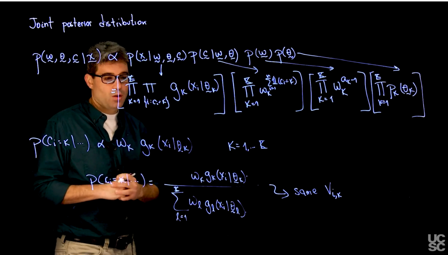
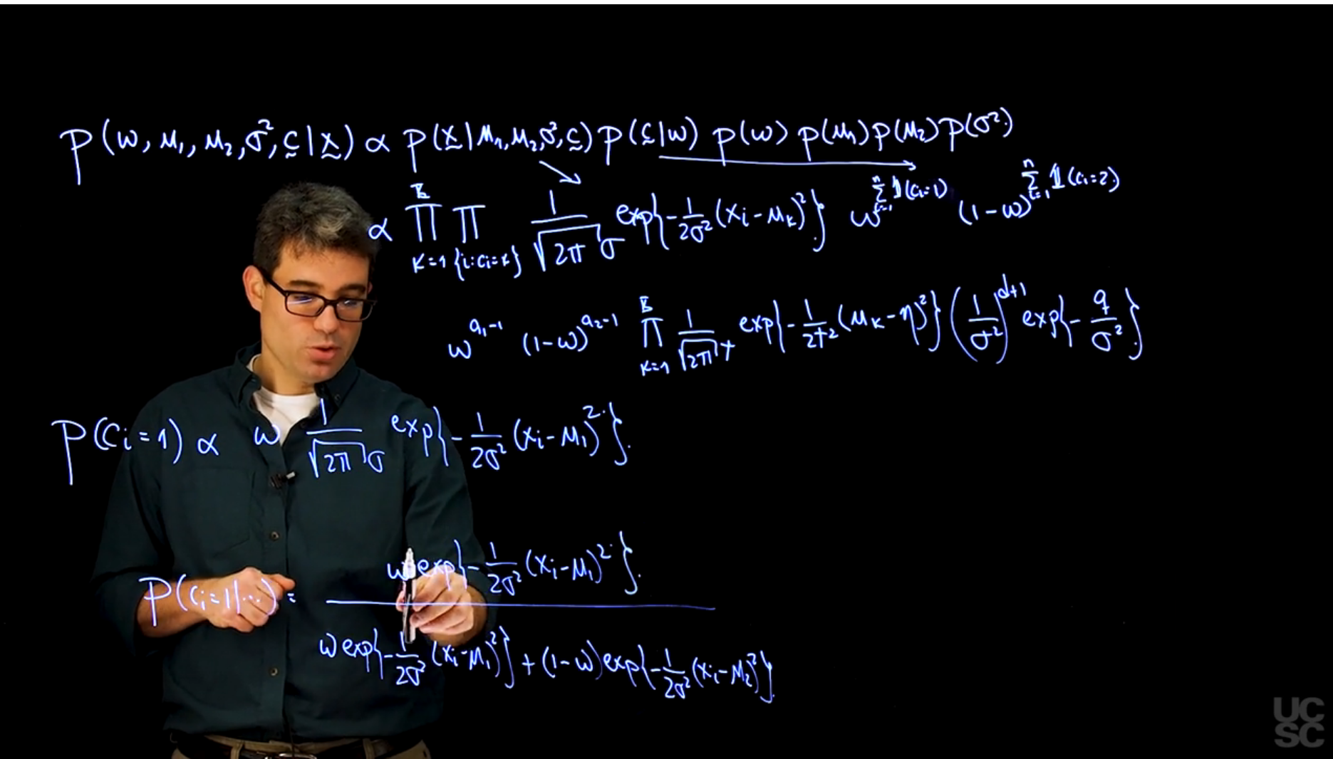
[So this provides a mirror image to what we did with the EM algorithm, but that has a Bayesian flavor rather than a frequentist flavor. Let's continue now with the full conditional posterior distribution for the indicators, for the c_is. I'm interested in the probability that c_i is equal to K given the data.]{.mark}
As before, this is going to be proportional to just the terms in this large product that depends on $c_i$, and if you look at it carefully, $c_i$ only appears in this two terms of the product.
These have nothing to do with $c_i.$
In particular, it appears in a single term within this really large product and in a single term within this product.
So the term that depends on $c_i$ being equal to $k$ in here is $\omega_k$.
The term that depends on
$c_i$ equal to $k$ in here, it's just $g_k(x_i \mid \theta_k)$, and this is true for
every $k$ from one to capital $K$.
Remember that $c_i$ is a discrete
random variable, taking values between one and $k$ because it indicates which component generated the observation.
So if I want to get rid of the proportionality sign and actually being able to write what the probability is, I just need to normalize this by dividing over the sum of these quantities over $k$.
So that means that $p(c_i = k \mid \text{all other parameters}) = \frac{\omega_k g_k(x_i \mid \theta_k)}{\sum_{l=1}^{K} \omega_l g_l(x_i \mid \theta_l)}$.
If you look at this expression carefully, you will realize that it is very similar to the expression that we used when computing in the EM algorithm, the weights associated which is one of the observations.
In fact, it is the same expression, and this is just what we called in the EM algorithm, $V_{ik}$. Finally, let's consider the full conditional posterior distribution for the data case.
So we need $p(\theta_k \mid \text{all other parameters})$.
Again, we just pick from this whole product the terms that have to do with $\theta_k$, in this case, it is the two in the middle that do
not depend on it, and within this big expression, we just have a few terms
that contain $\theta_k$, and those correspond to the observations that are currently assigned to that particular component.
So this expression is proportional to the product over the $i$'s that have been assigned to the $k$ th component of $g_k(x_i \mid \theta_k)$, and among this product, again, there is a single term that belongs to $\theta_k$.
So the form of the full conditional posterior distribution for the parameter $\theta_k$ is simply this.
Now, without a specific choice of $G$ and $P$, it is hard to further simplify this expression.
But what I do want to note here is that if this prior $p_k$ is conjugate to this kernel $g_k$, then we typically know what family this posterior
distribution will belong to, and that will make computation much simpler because you will typically be able to sample from that full posterior conditional distribution in using a direct sampler.
This will become a little bit more clear once we do an example with mixture models, which is what we're going to do next.
:::
## MCMC for location mixtures of normals Part 1
{#fig-s_06 .column-margin width="53mm" group="slides"}
{#fig-s_07 .column-margin width="53mm" group="slides"}
{#fig-s_08 .column-margin width="53mm" group="slides"}
{#fig-s_09 .column-margin width="53mm" group="slides"}
{#fig-s_10 .column-margin width="53mm" group="slides"}
\index{mixture!location mixture of normals}
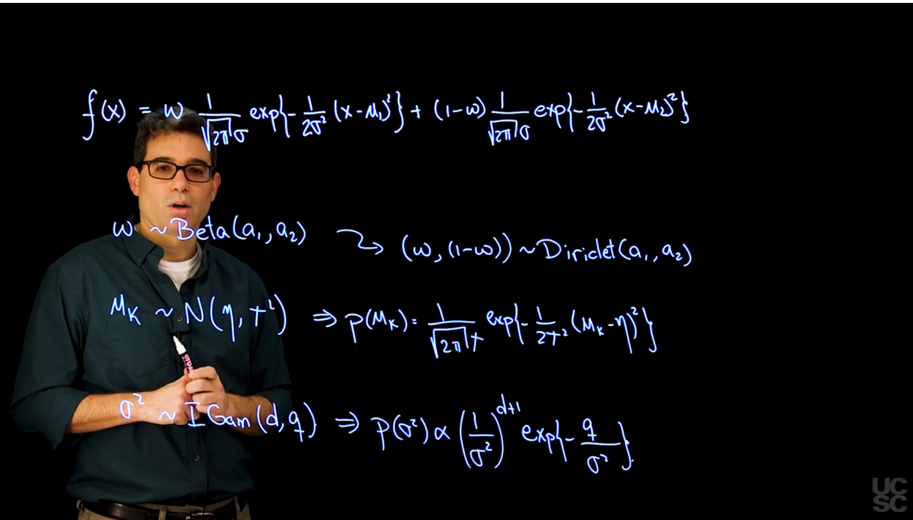
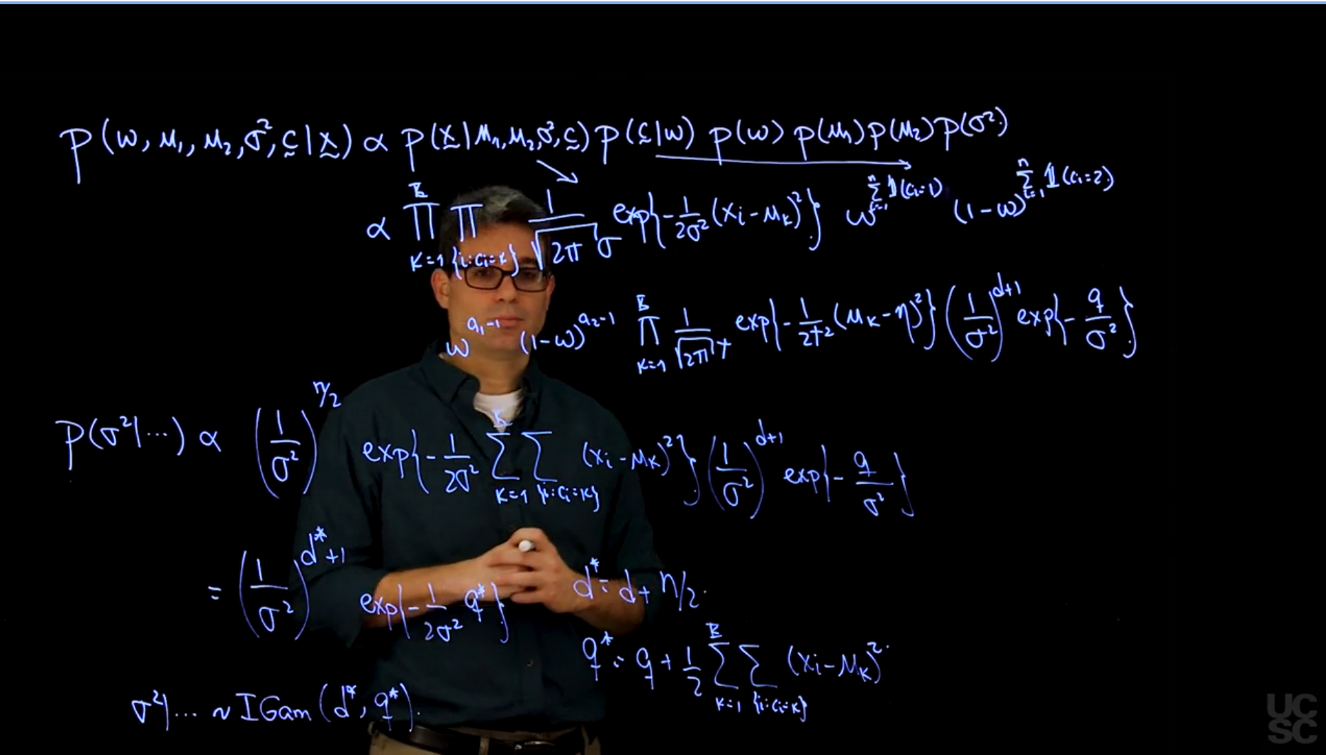
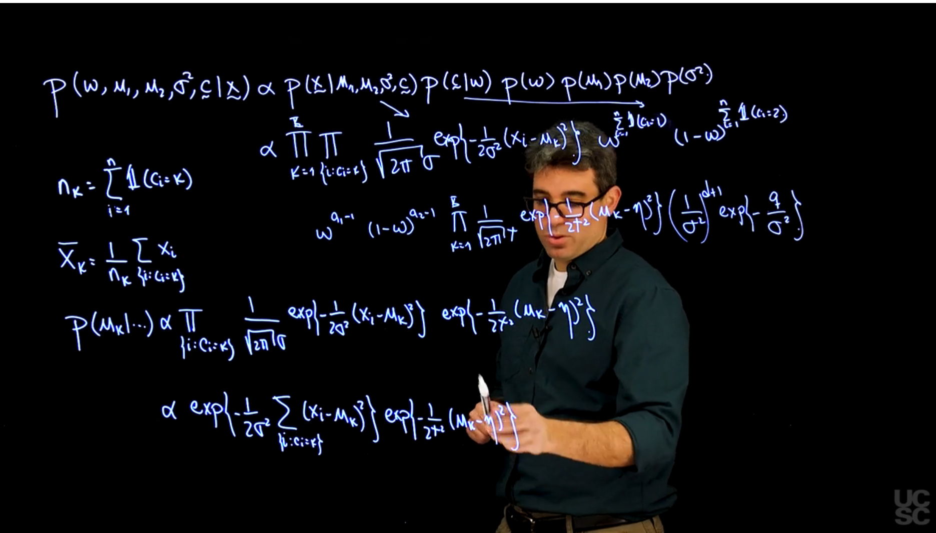
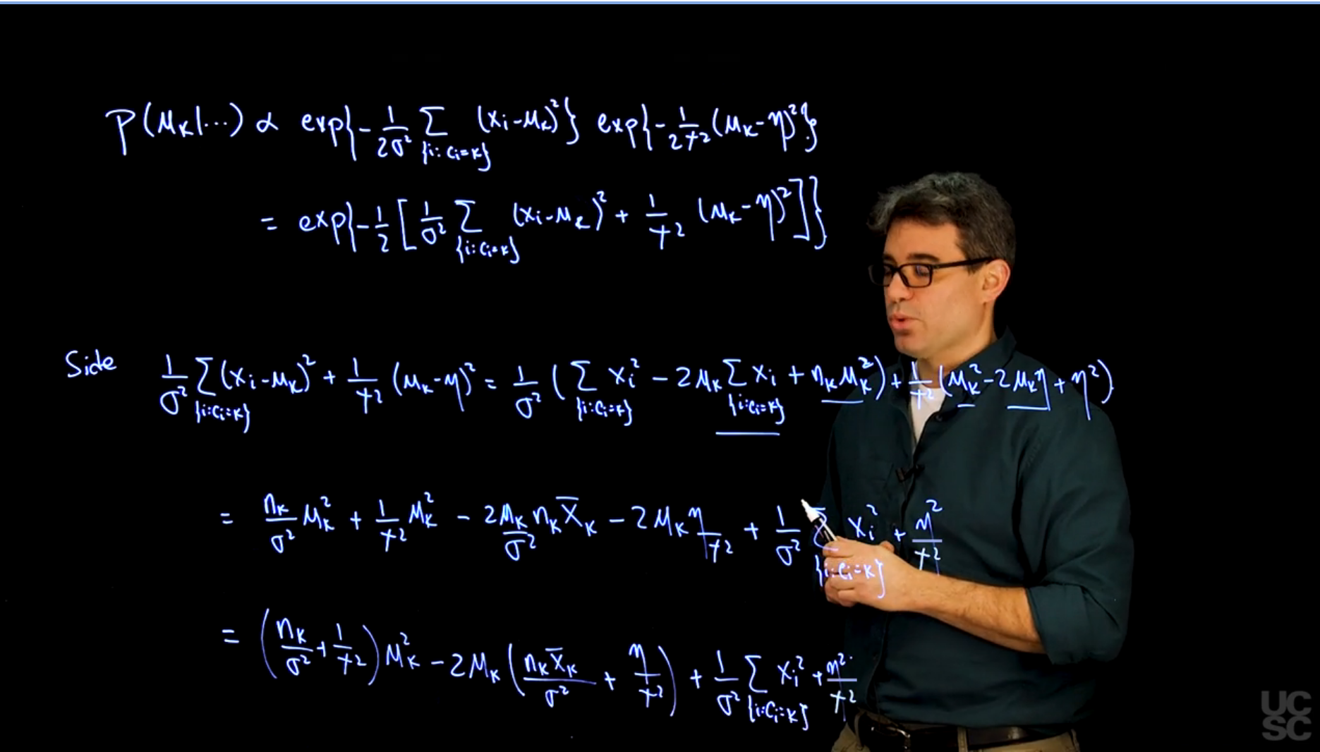
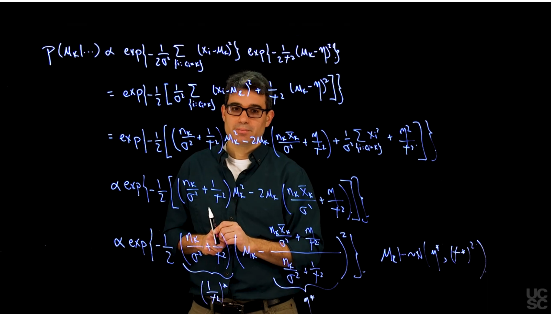
As in the previous module we derive the full conditional distributions for the mixture of two univariate normals.
$$
f(x \mid \omega, \mu_1, \mu_2, \sigma) = \omega \frac{1}{\sqrt{2\pi\sigma}} \exp\left\{-\frac{(x - \mu_1)^2}{2\sigma^2}\right\} + (1- \omega) \frac{1}{\sqrt{2\pi\sigma}} \exp\left\{-\frac{(x - \mu_2)^2}{2\sigma^2}\right\}
$$
we use a beta distribution with $a_1=1$ and $a_2=1$ for $\omega$
which corresponds to a uniform distribution and is a special case of a Dirichlet for $K=2$.
$\mu_k \sim \mathcal{N}(\eta,\tau^2)$
Inverse Gamma for $\sigma^2$ with shape parameter $a$ and scale parameter $b$.
An empirical approach to priors:
\index{mixture!empirical Bayes}
In the absence of real prior information we typically employ the observed data to guide the selection of the hyperparameter $\eta$, $\tau^2$, $d$ and $q$, in an approach that is reminiscent of empirical Bayes. In particular, we attempt to make the means of the different component lie in the same support of the observed data, so we take $\eta$ to be approximately equal the mean (or median) of the observations, and $\tau^2$ to be roughly equal to their variance. Similarly, for the prior on the variance $\sigma^2$ we set $d = 2$ (which implies that $\mathbb{E}(\sigma^2) = q$ and an infinite prior variance) and $q$ to be roughly equal to the variance of the observations. [Posteriors are often not very sensitive to changes on the prior means that remain within an order of magnitude of the values suggested above.]{.mark}
::: {.callout-note collapse="true"}
## Overthinking the priors
It seems that since this is a hierarchical model, we set the priors for different components from shared hyper-priors. This way the parameters can also be inferred and we can reduce the number of parameters we need to estimate !
:::
## MCMC for location mixtures of normals Part 2
{#fig-s_11 .column-margin width="53mm" group="slides"}
{#fig-s_12 .column-margin width="53mm" group="slides"}
{#fig-s_13 .column-margin width="53mm" group="slides"}
## MCMC Example 1
```{r}
#| label: lbl-mcmc-setup
#### Example of an MCMC algorithm for fitting a location mixture of 2 Gaussian components
#### The algorithm is tested using simulated data

## Clear the environment and load required libraries
rm(list=ls())
library(MCMCpack)
set.seed(81196) # So that results are reproducible
```
```{r}
#| label: lbl-mcmc-generate-data
## Generate data from a mixture with 2 components
KK         = 2
w.true     = 0.6  # True weights associated with the components
mu.true    = rep(0, KK)
mu.true[1] = 0   # True mean for the first component
mu.true[2] = 5   # True mean for the second component
sigma.true = 1   # True standard deviation of all components
n          = 120         # Number of observations to be generated
cc.true = sample(1:KK, n, replace=T, prob=c(w.true,1-w.true))
x  = rep(0, n)
for(i in 1:n){
  x[i] = rnorm(1, mu.true[cc.true[i]], sigma.true)
}
```
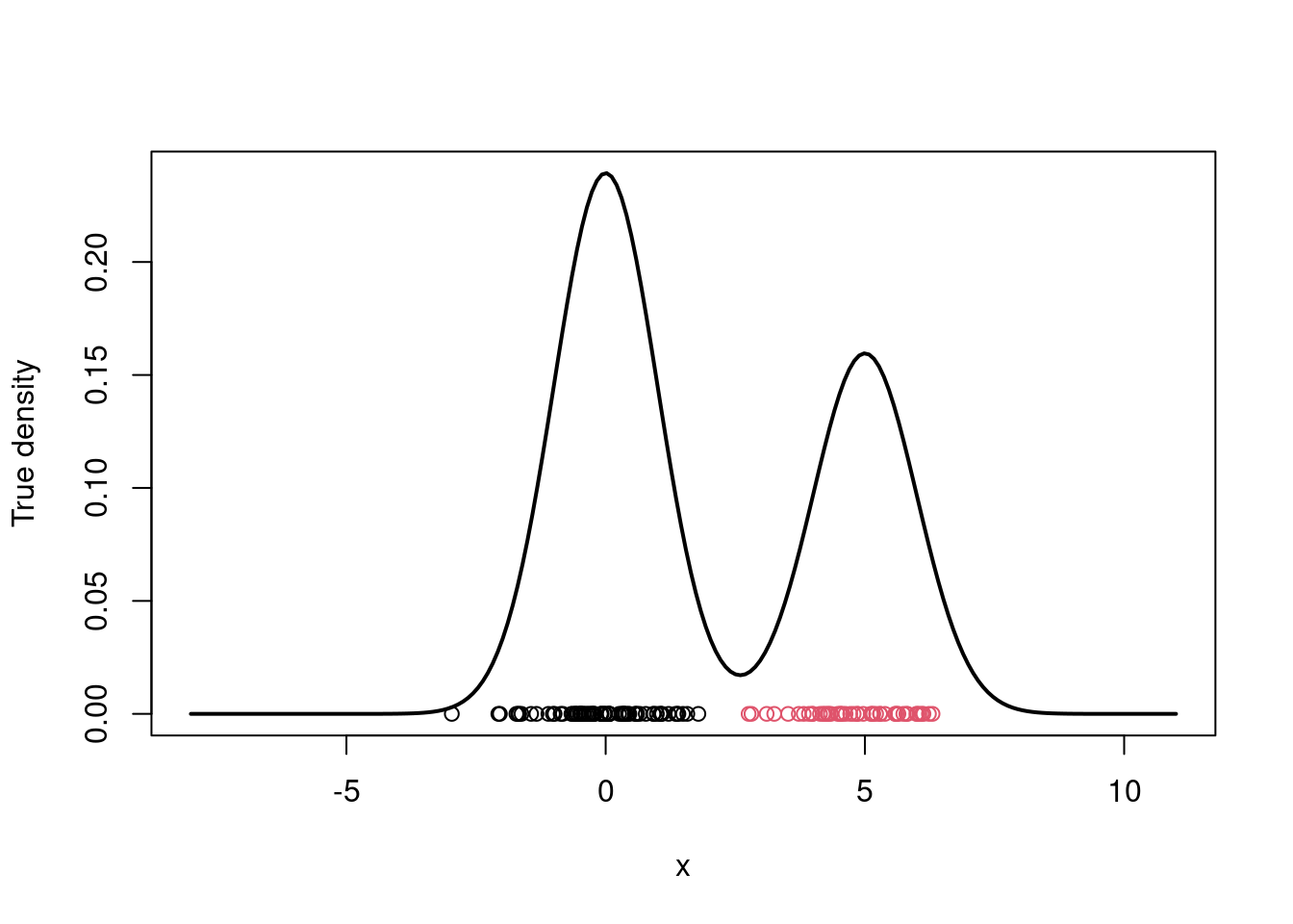
```{r}
#| label: fig-mcmc-true-density
#| fig-cap: "True density and data points"
# Plot the true density
par(mfrow=c(1,1))
xx.true = seq(-8,11,length=200)
yy.true = w.true*dnorm(xx.true, mu.true[1], sigma.true) +
  (1-w.true)*dnorm(xx.true, mu.true[2], sigma.true)
plot(xx.true, yy.true, type="l", xlab="x", ylab="True density", lwd=2)
points(x, rep(0,n), col=cc.true)
```
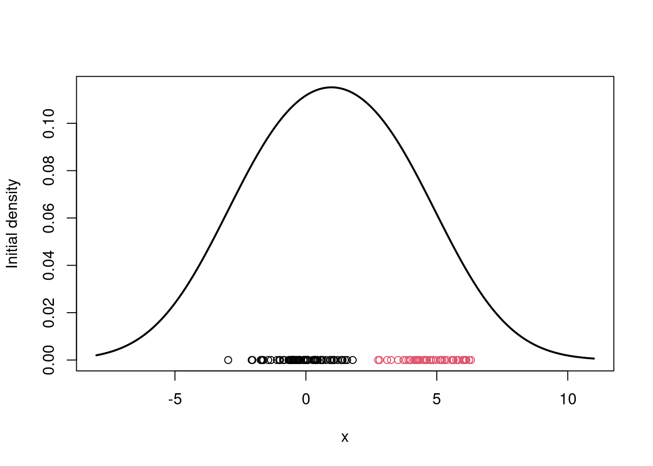
```{r}
#| label: lbl-mcmc-algorithm
## Initialize the parameters
w     = 1/2                         #Assign equal weight to each component to start with
mu    = rnorm(KK, mean(x), sd(x))   #Random cluster centers randomly spread over the support of the data
sigma = sd(x)                       #Initial standard deviation

# Plot the initial guess for the density
xx = seq(-8,11,length=200)
yy = w*dnorm(xx, mu[1], sigma) + (1-w)*dnorm(xx, mu[2], sigma)
plot(xx, yy, type="l", ylim=c(0, max(yy)), xlab="x",
     ylab="Initial density", lwd=2)
points(x, rep(0,n), col=cc.true)
## The actual MCMC algorithm starts here
# Priors
aa  = rep(1,KK)  # Uniform prior on w
eta = 0          # Mean 0 for the prior on mu_k
tau = 5          # Standard deviation 5 on the prior for mu_l
dd  = 2
qq  = 1

# Number of iterations of the sampler
rrr   = 6000
burn  = 1000


# Storing the samples
cc.out    = array(0, dim=c(rrr, n))
w.out     = rep(0, rrr)
mu.out    = array(0, dim=c(rrr, KK))
sigma.out = rep(0, rrr)
logpost   = rep(0, rrr)

# MCMC iterations
for(s in 1:rrr){
  # Sample the indicators
  cc = rep(0,n)
  for(i in 1:n){
    v = rep(0,KK)
    v[1] = log(w) + dnorm(x[i], mu[1], sigma, log=TRUE)  #Compute the log of the weights
    v[2] = log(1-w) + dnorm(x[i], mu[2], sigma, log=TRUE)  #Compute the log of the weights
    v = exp(v - max(v))/sum(exp(v - max(v)))
    cc[i] = sample(1:KK, 1, replace=TRUE, prob=v)
  }

  # Sample the weights
  w = rbeta(1, aa[1] + sum(cc==1), aa[2] + sum(cc==2))

  # Sample the means
  for(k in 1:KK){
    nk    = sum(cc==k)
    xsumk = sum(x[cc==k])
    tau2.hat = 1/(nk/sigma^2 + 1/tau^2)
    mu.hat  = tau2.hat*(xsumk/sigma^2 + eta/tau^2)
    mu[k]   = rnorm(1, mu.hat, sqrt(tau2.hat))
  }

  # Sample the variances
  dd.star = dd + n/2
  qq.star = qq + sum((x - mu[cc])^2)/2
  sigma = sqrt(rinvgamma(1, dd.star, qq.star))

  # Store samples
  cc.out[s,]   = cc
  w.out[s]     = w
  mu.out[s,]   = mu
  sigma.out[s] = sigma


  # Compute the log posterior
  for(i in 1:n){
    if(cc[i]==1){
      logpost[s] = logpost[s] + log(w) + dnorm(x[i], mu[1], sigma, log=TRUE)
    }else{
      logpost[s] = logpost[s] + log(1-w) + dnorm(x[i], mu[2], sigma, log=TRUE)
    }
  }

  logpost[s] = logpost[s] + dbeta(w, aa[1], aa[2],log = T)
  for(k in 1:KK){
    logpost[s] = logpost[s] + dnorm(mu[k], eta, tau, log = T)
  }

  logpost[s] = logpost[s] + log(dinvgamma(sigma^2, dd, 1/qq))

  # print s every 500 iterations
  if(s/500==floor(s/500)){
    print(paste("s =",s))
  }
}
```
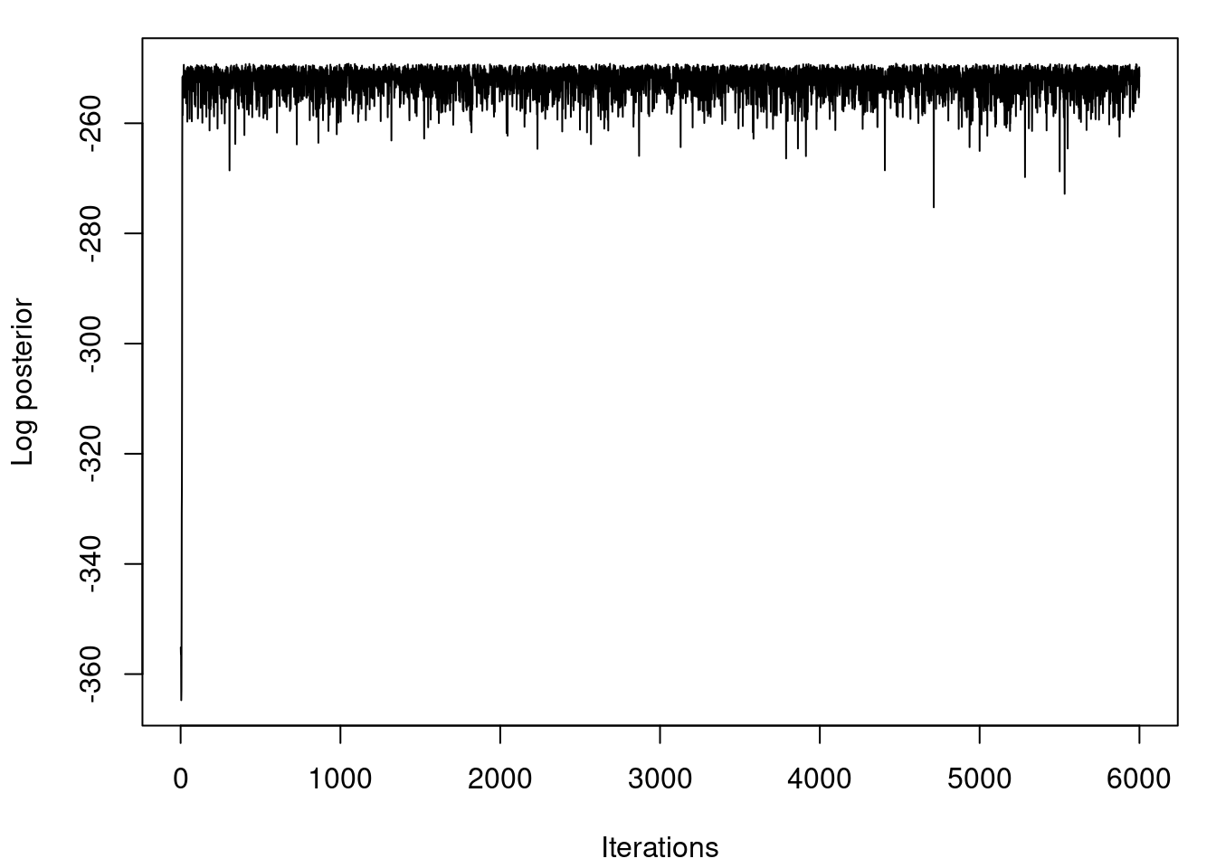
```{r}
#| label: fig-mcmc-plot-logpost
#| fig-cap: "Log posterior distribution for various samples"
## Plot the logposterior distribution for various samples
par(mfrow=c(1,1))
par(mar=c(4,4,1,1)+0.1)
plot(logpost, type="l", xlab="Iterations", ylab="Log posterior")

xx = seq(-8,11,length=200)
density.posterior = array(0, dim=c(rrr-burn,length(xx)))
for(s in 1:(rrr-burn)){
  density.posterior[s,] = density.posterior[s,] + w.out[s+burn]*dnorm(xx,mu.out[s+burn,1],sigma.out[s+burn]) +
                                                  (1-w.out[s+burn])*dnorm(xx,mu.out[s+burn,2],sigma.out[s+burn])
}
```
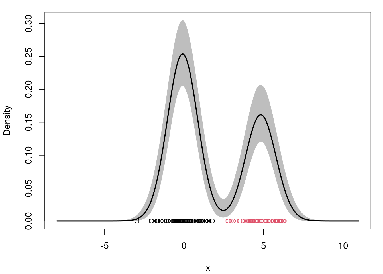
```{r}
#| label: fig-mcmc-plot-density
#| fig-cap: "Posterior density estimate"
## report the posterior mean and 95% credible interval
density.posterior.m = apply(density.posterior , 2, mean)
density.posterior.lq = apply(density.posterior, 2, quantile, 0.025)
density.posterior.uq = apply(density.posterior, 2, quantile, 0.975)

## Plot the posterior density estimate
par(mfrow=c(1,1))
par(mar=c(4,4,1,1)+0.1)
plot(xx, density.posterior.m, type="n",ylim=c(0,max(density.posterior.uq)), xlab="x", ylab="Density")
polygon(c(xx,rev(xx)), c(density.posterior.lq, rev(density.posterior.uq)), col="grey", border="grey")
lines(xx, density.posterior.m, lwd=2)
points(x, rep(0,n), col=cc.true)
```
## Sample code for MCMC example 1
## MCMC Example 2
## Sample code for MCMC example 2
```{r}
#| label: lbl-mcmc-example-2
#|
#### Example of an MCMC algorithm for fitting a mixtures of K p-variate Gaussian components
#### The algorithm is tested using simulated data

## Clear the environment and load required libraries
rm(list=ls())
library(mvtnorm)
library(ellipse)
library(MCMCpack)
## Generate data from a mixture with 3 components
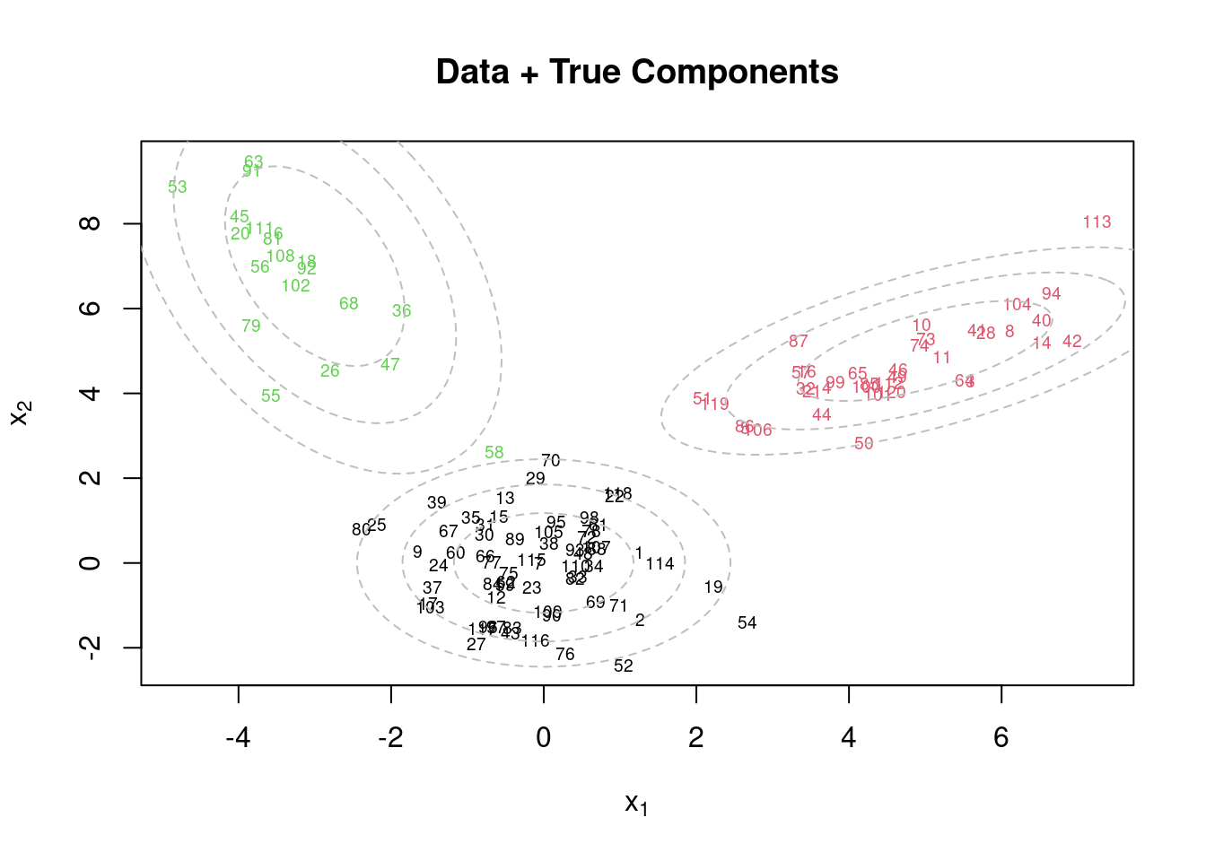
KK = 3
p = 2
w.true = c(0.5,0.3,0.2) # True weights associated with the components
mu.true = array(0, dim=c(KK,p))
mu.true[1,] = c(0,0) #True mean for the first component
mu.true[2,] = c(5,5) #True mean for the second component
mu.true[3,] = c(-3,7) #True mean for the third component
Sigma.true = array(0, dim=c(KK,p,p))
Sigma.true[1,,] = matrix(c(1,0,0,1),p,p) #True variance for the first component
Sigma.true[2,,] = matrix(c(2,0.9,0.9,1),p,p) #True variance for the second component
Sigma.true[3,,] = matrix(c(1,-0.9,-0.9,4),p,p) #True variance for the third component
set.seed(63252) #Keep seed the same so that we can reproduce results
n = 120
cc.true = sample(1:3, n, replace=T, prob=w.true)
x = array(0, dim=c(n,p))
for(i in 1:n){
x[i,] = rmvnorm(1, mu.true[cc.true[i],], Sigma.true[cc.true[i],,])
}
par(mfrow=c(1,1))
plot(x[,1], x[,2], col=cc.true, xlab=expression(x[1]), ylab=expression(x[2]), type="n")
text(x[,1], x[,2], seq(1,n), col=cc.true, cex=0.6)
for(k in 1:KK){
lines(ellipse(x=Sigma.true[k,,], centre=mu.true[k,], level=0.50), col="grey", lty=2)
lines(ellipse(x=Sigma.true[k,,], centre=mu.true[k,], level=0.82), col="grey", lty=2)
lines(ellipse(x=Sigma.true[k,,], centre=mu.true[k,], level=0.95), col="grey", lty=2)
}
title(main="Data + True Components")
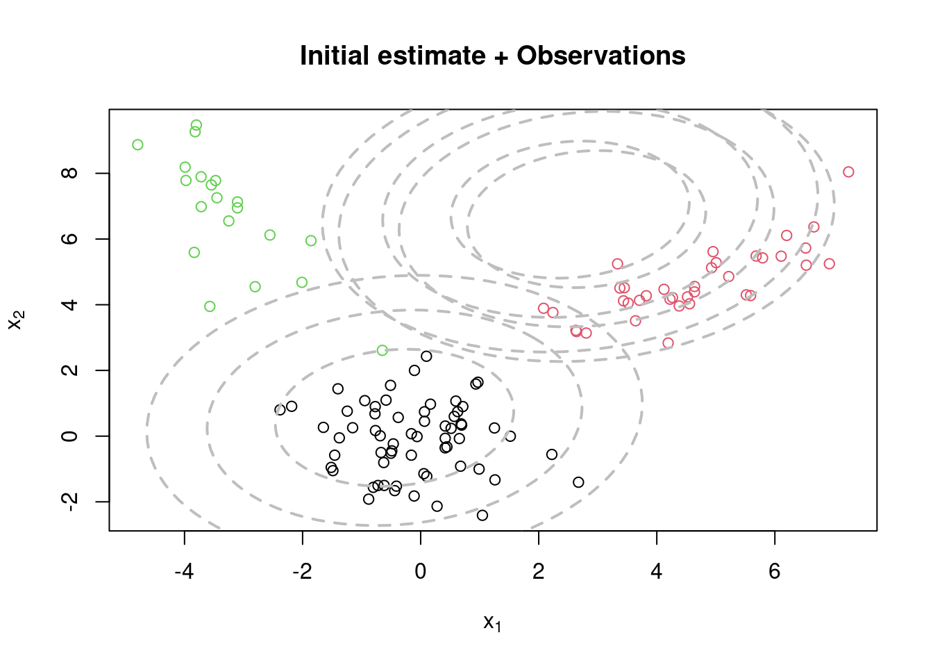
## Initialize the parameters
w          = rep(1,KK)/KK  #Assign equal weight to each component to start with
mu         = rmvnorm(KK, apply(x,2,mean), var(x))   #RandomCluster centers randomly spread over the support of the data
Sigma      = array(0, dim=c(KK,p,p))  #Initial variances are assumed to be the same
Sigma[1,,] = var(x)/KK
Sigma[2,,] = var(x)/KK
Sigma[3,,] = var(x)/KK
cc         = sample(1:KK, n, replace=TRUE, prob=w)

par(mfrow=c(1,1))
plot(x[,1], x[,2], col=cc.true, xlab=expression(x[1]), ylab=expression(x[2]))
for(k in 1:KK){
  lines(ellipse(x=Sigma[k,,], centre=mu[k,], level=0.50), col="grey", lty=2, lwd=2)
  lines(ellipse(x=Sigma[k,,], centre=mu[k,], level=0.82), col="grey", lty=2, lwd=2)
  lines(ellipse(x=Sigma[k,,], centre=mu[k,], level=0.95), col="grey", lty=2, lwd=2)
}
title(main="Initial estimate + Observations")
# Priors
aa = rep(1, KK)
dd = apply(x,2,mean)
DD = 10*var(x)
nu = p
SS = var(x)/3

# Number of iteration of the sampler
rrr = 1000

# Storing the samples
cc.out    = array(0, dim=c(rrr, n))
w.out     = array(0, dim=c(rrr, KK))
mu.out    = array(0, dim=c(rrr, KK, p))
Sigma.out = array(0, dim=c(rrr, KK, p, p))
logpost   = rep(0, rrr)

for(s in 1:rrr){
  # Sample the indicators
  for(i in 1:n){
    v = rep(0,KK)
    for(k in 1:KK){
      v[k] = log(w[k]) + mvtnorm::dmvnorm(x[i,], mu[k,], Sigma[k,,], log=TRUE)  #Compute the log of the weights
    }
    v = exp(v - max(v))/sum(exp(v - max(v)))
    cc[i] = sample(1:KK, 1, replace=TRUE, prob=v)
  }

  # Sample the weights
  w = as.vector(rdirichlet(1, aa + tabulate(cc)))

  # Sample the means
  DD.st = matrix(0, nrow=p, ncol=p)
  for(k in 1:KK){
    mk    = sum(cc==k)
    xsumk = apply(x[cc==k,], 2, sum)
    DD.st = solve(mk*solve(Sigma[k,,]) + solve(DD))
    dd.st = DD.st%*%(solve(Sigma[k,,])%*%xsumk + solve(DD)%*%dd)
    mu[k,] = as.vector(rmvnorm(1,dd.st,DD.st))
  }

  # Sample the variances
  xcensumk = array(0, dim=c(KK,p,p))
  for(i in 1:n){
    xcensumk[cc[i],,] = xcensumk[cc[i],,] + (x[i,] - mu[cc[i],])%*%t(x[i,] - mu[cc[i],])
  }
  for(k in 1:KK){
    Sigma[k,,] = riwish(nu + sum(cc==k), SS + xcensumk[k,,])
  }

  # Store samples
  cc.out[s,]      = cc
  w.out[s,]       = w
  mu.out[s,,]     = mu
  Sigma.out[s,,,] = Sigma
  for(i in 1:n){
    logpost[s] = logpost[s] + log(w[cc[i]]) + mvtnorm::dmvnorm(x[i,], mu[cc[i],], Sigma[cc[i],,], log=TRUE)
  }
  logpost[s] = logpost[s] + ddirichlet(w, aa)
  for(k in 1:KK){
    logpost[s] = logpost[s] + mvtnorm::dmvnorm(mu[k,], dd, DD, log=TRUE)
    logpost[s] = logpost[s] + log(diwish(Sigma[k,,], nu, SS))
  }

  if(s/250==floor(s/250)){
    print(paste("s = ", s))
  }
}
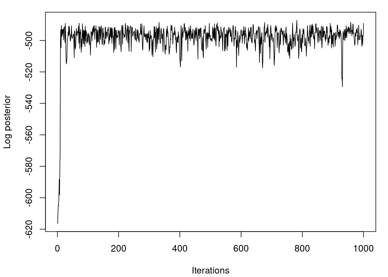
## Plot the logposterior distribution for various samples
par(mfrow=c(1,1))
par(mar=c(4,4,1,1)+0.1)
plot(logpost, type="l", xlab="Iterations", ylab="Log posterior")
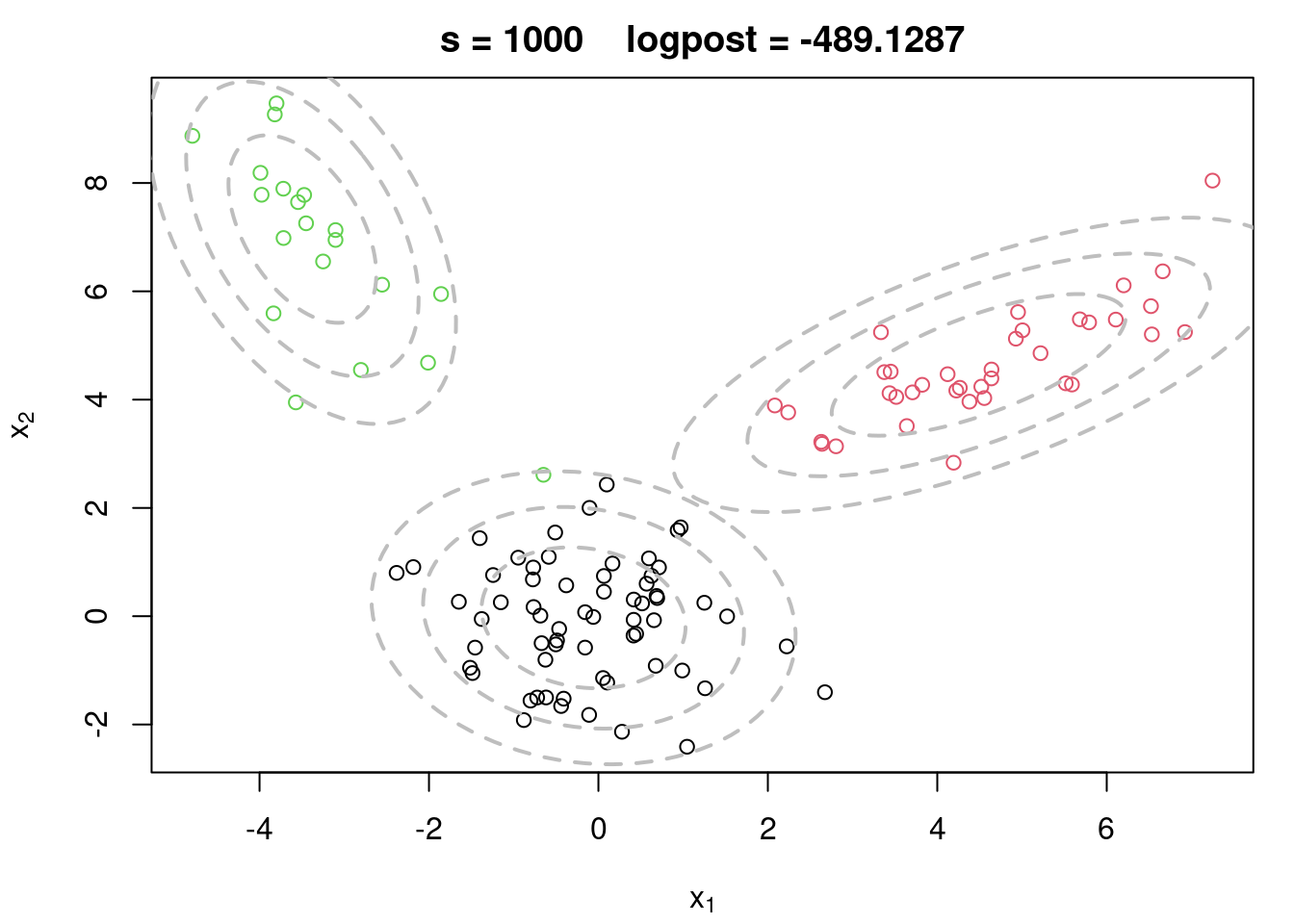
## Plot the density estimate for the last iteration of the MCMC
par(mfrow=c(1,1))
par(mar=c(4,4,2,1)+0.1)
plot(x[,1], x[,2], col=cc.true, main=paste("s =",s,"   logpost =", round(logpost[s],4)), xlab=expression(x[1]), ylab=expression(x[2]))
for(k in 1:KK){
  lines(ellipse(x=Sigma[k,,], centre=mu[k,], level=0.50), col="grey", lty=2, lwd=2)
  lines(ellipse(x=Sigma[k,,], centre=mu[k,], level=0.82), col="grey", lty=2, lwd=2)
  lines(ellipse(x=Sigma[k,,], centre=mu[k,], level=0.95), col="grey", lty=2, lwd=2)
}
```
## Practice Graded Assignment: The MCMC algorithm for zero-inflated mixtures
```{r}
#| label: mcmc_zero_inflated
rm(list=ls())
library(MCMCpack)
set.seed(81196)  # So that results are reproducible

# Data loading

x <- read.csv("./data/nestsize.csv")[[1]]
n <- length(x)

# The actual MCMC algorithm starts here

## MCMC iterations of the sampler

iterations <- 6000
burn <- 1000

## Initialize the parameters

cc         = rep(2, n)
cc[x == 0] = sample(1:2, sum(x == 0), replace = TRUE, prob = c(0.5, 0.5))

## Priors

aa = c(1, 1)  # Uniform prior on w
w     = 0.2 # fewer zeros
lambda = mean(x[x > 0])  # Initial lambda from nonzero data

# Storing the samples
w.out      = rep(0, iterations)
cc.out     = array(0, dim=c(iterations, n))
lambda.out = array(0, dim=c(iterations, n))

# logpost    = rep(0, iterations)
# MCMC iterations

for (s in 1:iterations) {

  # Sample latent indicators c_i

  cc = numeric(n)
  for (i in 1:n) {
    if (x[i] == 0) {
      logp1 = log(w)
      logp2 = log(1 - w) + dpois(0, lambda, log=TRUE)
      probs = exp(c(logp1, logp2) - max(logp1, logp2))
      probs = probs / sum(probs)
      cc[i] = sample(1:2, 1, prob = probs)
    } else {
      cc[i] = 2
    }
  }

  # Sample the weights

  w = rbeta(1, aa[1] + sum(cc==1), aa[2] + sum(cc==2))
  lambda = rgamma(1, shape = 1 + sum(x[cc == 2]), rate = 1 + sum(cc == 2))

  # Store samples

  w.out[s] =  w
  lambda.out[s]  = lambda
  cc.out[s,] = cc

}

# Posterior summaries

w.post = w.out[-(1:burn)]
lambda.post = lambda.out[-(1:burn)]
cat("Posterior mean of w:", mean(w.post), "\n")
cat("Posterior mean of lambda:", mean(lambda.post), "\n")
```
## Honors Peer-graded Assignment: Markov chain Monte Carlo algorithms for Mixture Models