Y_i \sim \mathrm{Poisson}(\lambda) \tag{18.1}
The likelihood of the data is given by the Poisson distribution.
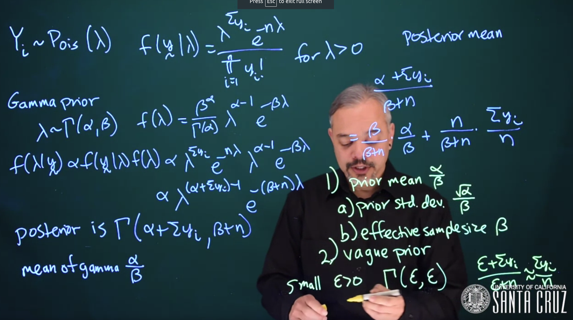
\begin{aligned} {\color{red}f(y \mid \lambda) = \frac{\lambda^{\sum{y_i}}e^{-n\lambda}}{\prod_{i = 1}^n{y_i!}}} \quad \forall (\lambda > 0) && \text{ Poisson Likelihood } \end{aligned}
It would be convenient if we could put a conjugate prior. What distribution looks like \lambda raised to a power and e raised to a negative power?
For this, we’re going to use a Gamma prior.
\begin{aligned} \lambda &\sim \mathrm{Gamma}(\alpha, \beta) && \text{Gamma Prior} \\ \color{green}{ f(\lambda)} &= \color{green}{\frac{\beta^\alpha}{\Gamma(\alpha)}\lambda^{\alpha - 1}e^{-\beta\lambda}} && \text{subst. Gamma PDF} \end{aligned} \tag{18.2}
We can use Bayes theorem to find the posterior.
\begin{aligned} {\color{blue}f(\lambda \mid y)} &\propto \color{red}{ f(y \mid \lambda)} \color{green}{ f(\lambda)} && \text{Bayes without the denominator} \\ &\propto \color{red}{\lambda^{\sum{y_i}}e^{-n\lambda}}\color{green}{\lambda^{\alpha - 1}e^{-\beta \lambda} } && \text{subst. Likelihood and Prior} \\ & \propto { \color{blue} \lambda^{\alpha + \sum{y_i} - 1}e^{-(\beta + n)\lambda} } && \text{collecting terms} \\ & \propto { \color{blue} \mathrm{Gamma}(\alpha + \sum{y_i}, \beta + n)} \end{aligned} \tag{18.3}
The posterior is a Gamma distribution with parameters \alpha + \sum{y_i} and \beta + n.
Thus we can see that the posterior is a Gamma Distribution
\lambda \mid y \sim \mathrm{Gamma}(\alpha + \sum{y_i}, \beta + n) \tag{18.4}
The posterior mean of a Gamma distribution is given by
The mean of Gamma under this parameterization is: \frac{\alpha}{\beta}
The posterior mean is going to be
\begin{aligned} {\color{blue}\mu_{\lambda}} &= \frac{\alpha + \sum{y_i}}{\beta + n} && \text{(Posterior Mean)} \\ posterior_{\mu} &= \frac{\alpha + \sum{y_i}}{\beta + n} \\ &= \frac{\beta}{\beta + n}\frac{\alpha}{\beta} + \frac{n}{\beta + n}\frac{\sum{y_i}}{n} \\ & \propto \beta \cdot \mu_\text{prior} + n\cdot \mu_\text{data} \end{aligned} \tag{18.5}
The posterior variance of a Gamma distribution is given by
As you can see here the posterior mean of the Gamma distribution is also the weighted average of the prior mean and the data mean.
Therefore, the effective sample size (ESS) of the Gamma prior is \beta
Here are two strategies for choose the hyper-parameters \alpha and \beta
- An informative prior with a prior mean guess of \mu=\frac{a}{b} e.g. what is the average number of chips per cookie?
- Next we need another piece of knowledge to pinpoint both parameters.
- Can you estimate the error for the mean? I.e. what do you think the standard deviation is? Since for the Gamma prior
- What is the effective sample size \text{ESS}=\beta ?
- How many units of information do you think we have in our prior v.s. our data points ? \sigma = \frac{ \sqrt{\alpha} }{\beta}
- A vague prior refers to one that’s relatively flat across much of the space.
- For a Gamma prior we can choose \Gamma(\varepsilon, \varepsilon) where \varepsilon is small and strictly positive. This would create a distribution with a \mu = 1 and a huge \sigma stretching across the whole space. And the effective sample size will also be \varepsilon Hence the posterior will be largely driven by the data and very little by the prior.
The first strategy with a mean and an ESS will be used in numerous models going forward so it is best to remember these two strategies!