seq(from=0.1, to = 0.9, by = 0.1)[1] 0.1 0.2 0.3 0.4 0.5 0.6 0.7 0.8 0.9Distributions, Bernoulli Distribution, Binomial Distribution
Before delving into Bayesian inference in the next module, in this module we will review inference in the frequentist approach. Much of the material was developed by R. A. Fischer in the last century. Some of the central ideas and tools of this approach include:
One point of interest is how much of this work is based on the law of large numbers, central limit theorem and the empirical rule, three related key results in probability theory.
However the second point to stress is that the frequentist paradigm is fraught with practical as well as philosophical challenges which are handled better to some extent within the Bayesian paradigm.
In particular, the frequentist paradigm does not allow us to make probability statements about parameters, which is a key feature of the Bayesian approach.
A brief review of the frequentist approach to inference will be useful for contrasting with the Bayesian approach. (Kruschke 2011) Chapter 2 suggests that CI provides the basis for a Bayesian workflow and that the rest of the text fills in the missing pieces.
Under the frequentist paradigm, one views the data as a random sample from some larger, potentially hypothetical population. We can then make probability statements i.e. long-run frequency statements based on this larger population.
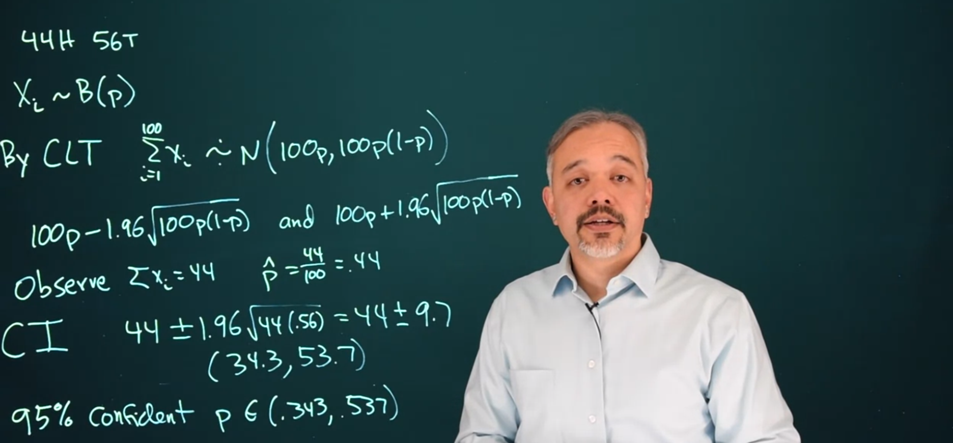
Example 9.1 (Coin Flip Example - Central Limit Theorem) Suppose we flip a coin 100 times. And we get 44 heads and 56 tails. We can view these 100 flips as a random sample from a much larger infinite hypothetical population of flips from this coin. We can say that each flip is X_i an RV which follows a Bernoulli distribution with some probability p. In this case p is unknown, but we can assume it is fixed since we are using a specific physical coin.
X_i \sim B(p) \tag{9.1}
We ask :
To estimate p we will apply the Central limit theorem c.f. Central Limit Theorem which states that the mean of a large number of IID RV with mean \mu and variance \sigma^2 is approximately N(\mu,\sigma^2).
\sum^{100}_{i=1} X_i\mathrel{\dot \sim } \mathcal{N}(100 \enspace p, 100 \enspace \mathbb{P}r(1-p)) \tag{9.2}
Given that this is a Normal distribution, we can use the empirical rule often called the 68-95-99.7 rule see (Wikipedia contributors 2023), that says 95% of the time we will get a result is in within 1.96 standard deviations of the mean. This is referred to as a Confidence Interval or (CI).
95\% \: \text{CI}= 100 \: \hat{p} \pm 1.96\sqrt{100 \: \hat{p}(1-\hat{p})} \tag{9.3}
Since we observed 44 heads we can estimate \hat{p} as
\hat p = \frac{44}{100} = .44 \tag{9.4}
This answers our first questions. Now we want to quantify our uncertainty.
\begin{aligned} 95\% \: \text{CI for 100 tosses} &= 100 \: (.44) \pm 1.96\sqrt{100(0.44)(1-0.44)} \\ &= 44 \pm 1.96\sqrt{(44) (0.56)} \\ &= 44 \pm 1.96\sqrt{23.64} \\ &= (34.27,53.73) \end{aligned} \tag{9.5}
We can be 95% confident that 100\times \hat{p} \in [34.3,53.7] We can say that we’re 95% confident that the true probability p \in (.343, .537).
If one were to ask do I think this coin is Fair ? This is a reasonable hypothesis, since 0.5 \in [.343,.537].
But we can also step back and say what does this interval mean when we say we’re 95% confident? Under the frequentist paradigm, we have to think back to our infinite hypothetical sequence of events, were we to repeat this trial an arbitrarily large number of times and each time create a confidence interval, then on average 95% of the intervals we make will contain the true value of p. This makes senses as a long run frequency explanation.
On the other hand, we might want to know something about this particular interval. Does this interval contain the true p. What’s the probability that this interval contains a true p? Well, we don’t know for this particular interval. But under the frequentist paradigm, we’re assuming that there is a fixed right answer for p. Either p is in that interval or it’s not in that interval. And so technically, from a frequentist perspective, the probability that p is in this interval is either 0 or 1. This is not a particularly satisfying explanation. In the other hand when we get to the Bayesian approach we will be able to compute an interval and actually say there is probably a p is in this interval is 95% based on a random interpretation of an unknown parameter.
In this example of flipping a coin 100 times, observing 44 heads resulted in the following 95% confidence interval for p: (.343, .537). From this, we concluded that it is plausible that the coin may be fair because p=.5 is in the interval.
Suppose instead that we flipped the coin 100,000 times, observing 44,000 heads (the same percentage of heads as before). Then using the method just presented, the 95% confidence interval for p is (.437, .443). Is it still reasonable to conclude that this is a fair coin with 95% confidence?
No Because 0.5 \not\in (.437, .443), we must conclude that p=.5 is not a plausible value for the population mean . Observing 100,000 flips increases the power of the experiment, leading to a more precise estimate with a narrower CI, due to the law of large numbers.
Example 9.2 (Heart Attack Patients - MLE) Consider a hospital where 400 patients are admitted over a month for heart attacks, and a month later 72 of them have died and 328 of them have survived.
Under the frequentist paradigm, we must first establish our reference population. This is the cornerstone of our thinking as we are considering how the sample parameter approximates the population statistic. What do we think our reference population is here?
Both Ref Pop 1 and Ref Pop 2 seem like viable options. Unfortunately, in our data is not a random sample drawn from either. We could pretend they are and move on, or we could also try to think harder about what our data is sampled from, perhaps Ref Pop 3.
This is an odd hypothetical situation, and so there are some philosophical issues with the setup of this whole problem within the frequentist paradigm
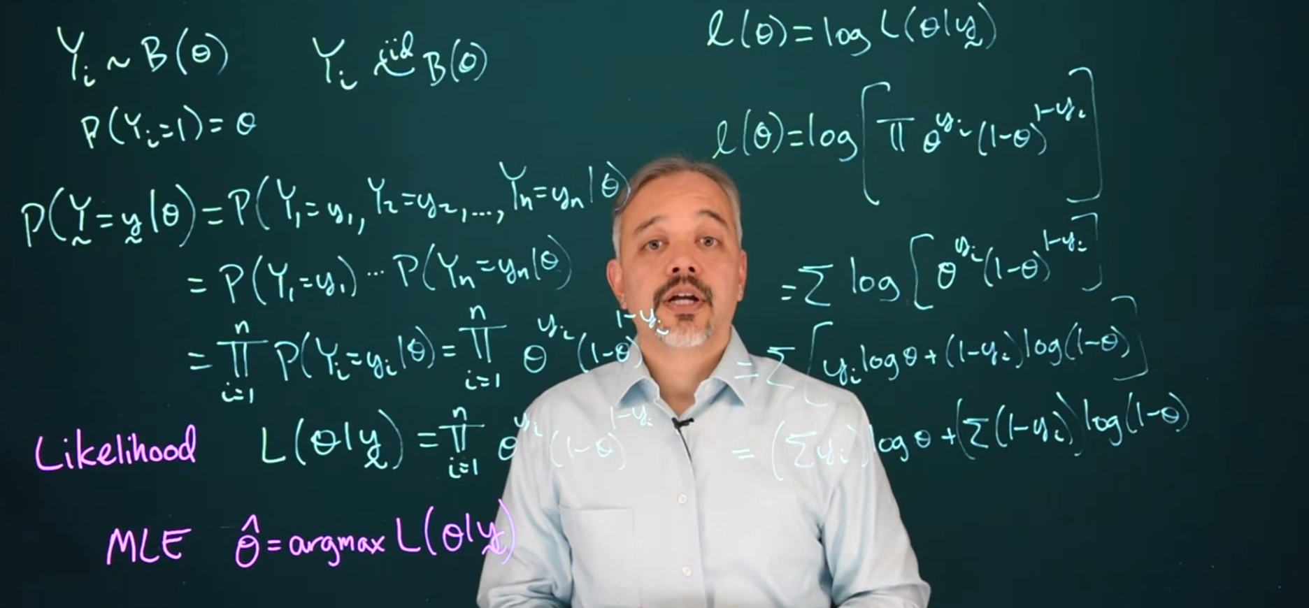
Y_i \sim \mathrm{Bernoulli}(p) \tag{9.6}
Since this is a Bernoulli trial we need to specify what we interpret as the success . In this case, the success is a mortality.
\mathbb{P}r(Y_i=1) = \theta \tag{9.7}
The PDF for the dataset can be written in vector form. \mathbb{P}r(\vec{Y}=\vec{y} \mid \theta) is the Probability of all the Y’s take some value little y given a value of theta.
\begin{aligned} \mathbb{P}r(\vec{Y}=\vec{y} \mid \theta) &= \mathbb{P}r(Y_1=y,\dots,Y_n=y_n \mid \theta) && \text{(joint probability)}\\ &= \mathbb{P}r(Y_1=y_1 \mid \theta) \cdots \mathbb{P}r(Y_n=y_n \mid \theta) && \text {(independence)}\\ &= \prod^n_{i=1} \mathbb{P}r(Y_i=y_i \mid \theta) && \text {(product notation)}\\ &= \prod^n_{i=1} \theta^{y_i} (1-\theta)^{1-y_i} && \text {(Bernoulli PMF)} \end{aligned} \tag{9.8}
We now cal the expression for \mathbb{P}r(\vec{Y}=\vec{y} \mid \theta) above the likelihood function L(\theta \mid \vec{y} ):
\mathcal{L}(\theta\mid\vec{y}) = \prod^n_{i=1} \theta^{y_i} (1-\theta)^{1-y_i} \tag{9.9}
Recall that we want to find the mortality rate parameter \theta for our Sample \vec Y.
Since it is a probability, it has a range of values from 0 to 1. One way to estimate it is that there should be one value that maximizes (Equation 9.9). It makes the data the most likely to occur for the particular data we observed. This is referred to as the maximum likelihood estimate (MLE).
\mathop{\mathrm{MLE}}(\hat \theta) = \mathop{\mathrm{argmax}} \; \mathcal{L}(\theta\mid y) \tag{9.10}
Although we are trying to find the \theta that maximizes the likelihood, in practice, it’s usually easier to maximize the natural logarithm of the likelihood, commonly referred to as the log-likelihood.
\begin{aligned} \mathcal{L}(\theta) &= \log(L(\theta|\vec{y})) && \\ &= \log(\prod^n_{i=1} {\theta^{y_i} (1-\theta)^{1-y_i}}) && \text{subst. likelihood} \\ &= \sum^n_{i=1}{ \log(\theta^{y_i}) + \log(1-\theta)^{1-y_i}} && \text{log product rule} \\ &= \sum^n_{i=1}{ y_i \log(\theta) + (1-y_i) \log(1-\theta)} && \text{log power rule}\\ &= \log(\theta) \sum^n_{i=1}{ y_i + \log(1-\theta)} \sum^n_{i=1}{ (1-y_i) }& & \text{extracting logs} \end{aligned} \tag{9.11}
What is the interpretation of the MLE of \theta in the context of the heart attack example?
If \hat \theta is the MLE for \theta, the 30-day mortality rate, then all possible values of \theta produce a lower value of the likelihood than \hat \theta.
To calculate the MLE one should differentiate \mathcal{L}(\theta) w.r.t. \theta and then set it equal to 0.
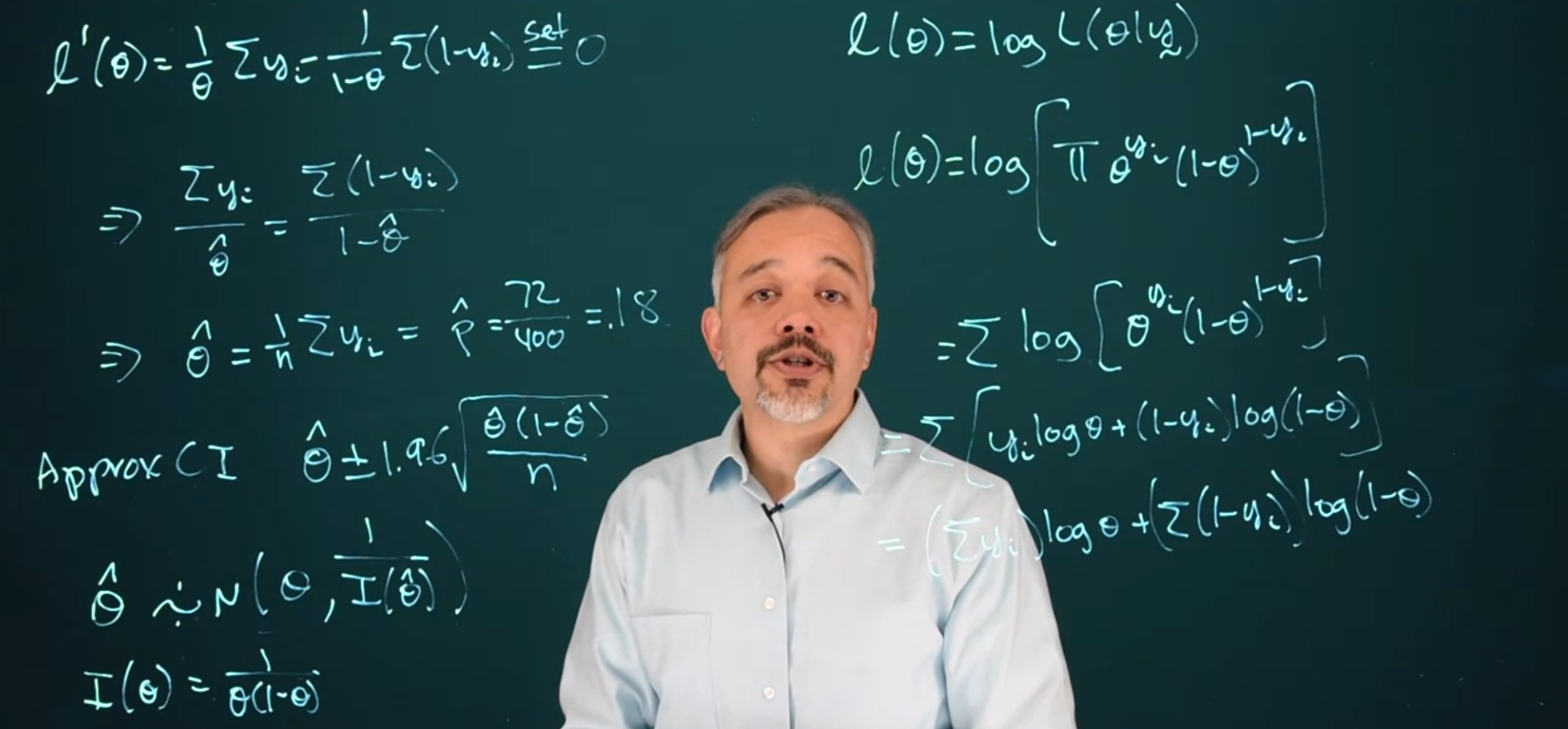
\begin{aligned} && \mathcal{L}'(\theta)=& \frac{1}{\theta}\sum_{i=1}^n y_i-\frac{1}{1-\theta}\sum_{i=1}^n 1-y_i \stackrel{\text{set}}{=}0 \text { set derivative to 0} \\ & \implies & \frac{1}{\hat \theta}\sum_{i=1}^n y_i & = \frac{1}{1- \hat \theta}\sum_{i=1}^n 1 - y_i \\ & \implies & (1 -\hat \theta) \sum_{i=1}^n{y_i} &= \hat\theta \sum_{i=1}^n {1-y_i} \\ & \implies & 1 \sum_{i=1}^n{y_i} - \cancel{ \hat \theta \sum_{i=1}^{n}{y_i}} &= \hat\theta \sum_{i=1}^n {1} - \cancel{\hat\theta \sum_{i=1}^n {y_i}} \\ & \implies & \sum_{i=1}^n{y_i} &= \hat\theta N \\ & \implies & \hat \theta &= \frac{1}{N} \sum_{i=1}^n y_i = \hat p = \frac{72}{400}=.18 \end{aligned}
Maximum Likelihood Estimates (MLEs) possess the following favorable properties:
using the Central Limit theorem (see Theorem F.1).
\hat \theta \pm 1.96\sqrt\frac{\hat \theta(1-\hat \theta)}{n}
\hat \theta \simeq \mathcal{N}(\theta,\frac{1}{\mathcal{I} (\hat \theta)})
where \mathcal{I} is the Fischer information which for the Bernoulli distribution is:
\mathcal{I}( \hat \theta) = \frac{1}{\theta(1-\theta)}
Note: The Fischer information is a measure of how much information about theta is in each data point!
In XAI we use discuss local and global explanations.
Global explanations explain a black box model’s predictions based on each feature, via its parameters.Local explanations explain the prediction of a specific datum from its features.since Fischer information quantifies the information in a data point on a parameter we should be able to use it to produce local and perhaps even global explanations for Bayesian models.
Some more examples of maximum likelihood estimators.

Let’s say X_i are exponential distributed
X_i \sim \mathrm{Exp}(\lambda)
Let’s say the data is independent and identically distributed, therefore making the overall density function
\begin{aligned} f(x \mid \lambda) &= \prod_{i = 1}^n{\lambda e^{-\lambda x_i}} && \text {(simplifying)} \\ &= \lambda^ne^{-\lambda \sum{x_i}} \end{aligned} \tag{9.12}
Now the likelihood function is
\mathcal{L}(\lambda \mid x)=\lambda^ne^{-\lambda \sum{x_i}} \tag{9.13}
the log likelihood is
\ell(\lambda) = n\ln{\lambda} - \lambda\sum_i{x_i} \tag{9.14}
Taking the derivative
\begin{aligned} \ell^\prime(\lambda) &= \frac{n}{\lambda} - \sum_i{x_i} \stackrel{\text{set}}{=}0 && \text {(set derivative = 0)} \\ \implies \frac{n}{\hat{\lambda}} &= \sum_i{x_i} && \text{(rearranging)} \end{aligned} \tag{9.15}
\hat{\lambda} = \frac{n}{\sum_i{x_i}} = \frac{1}{\bar{x}} \tag{9.16}
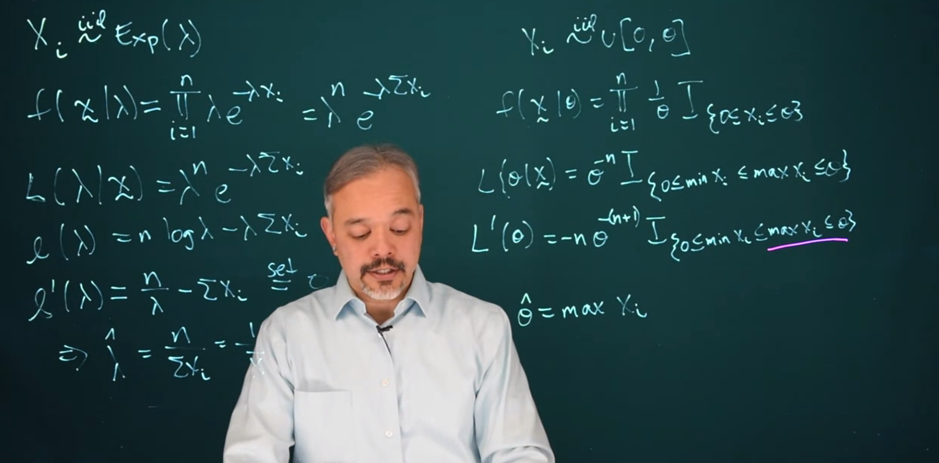
X_i \sim \mathcal{U}[0, \theta] \tag{9.17}
f(x \mid \theta) = \prod_{i = 1}^n{\frac{1}{\theta}\mathbb{I}_{0 \le x_i \le \theta}} \tag{9.18}
Combining all the indicator functions, for this to be a 1, each of these has to be true. These are going to be true if all the observations are bigger than 0, as in the minimum of the x is bigger than or equal to 0. The maximum of the x’s is also less than or equal to \theta.
\mathcal{L}(\theta|x) = \theta^{-1} \mathbb{I}_{0\le min(x_i) \le max(x_i) \le \theta} \tag{9.19}
\mathcal{L}^\prime(\theta) = -n\theta^{-(n + 1)}\mathbb{I}_{0 \le min(x_i) \le max(x_i)\le \theta} \tag{9.20}
We ask, can we set this equal to zero and solve for \theta? It turns out, this is not equal to zero for any \theta positive value. We need \theta to be strictly larger than zero. But for \theta positive, this will always be negative. The derivative is negative, that says this is a decreasing function. Therefore this function will be maximized when we pick \theta as small as possible. What’s the smallest possible value of \theta we can pick? Well we need in particular for \theta to be larger than all of the X_i. And so, the maximum likelihood estimate is the maximum of X_i
\hat{\theta} = max(x_i) \tag{9.21}
The cumulative distribution function (CDF) exists for every distribution. We define it as F(x) = \mathbb{P}r(X \le x) for random variable X.
If X is discrete-valued, then the CDF is computed with summation F(x) = \sum_{t = -\infty}^x {f(t)}. where f(t) = \mathbb{P}r(X = t) is the probability mass function (PMF) which we’ve already seen.
If X is continuous, the CDF is computed with an integral F(x) = \int_{-\infty}^x{f(t)dt}
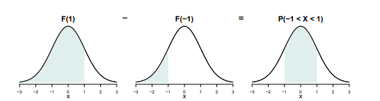
The CDF is convenient for calculating probabilities of intervals. Let a and b be any real numbers with a < b. Then the probability that X falls between a and b is equal to \mathbb{P}r(a < X < b) = \mathbb{P}r(X \le b) - \mathbb{P}r(X \le a) = F(b) - F(a)
Example 9.3 (CDF example 1) Suppose X \sim \mathrm{Binomial}(5, 0.6). Then
\begin{aligned} F(1) &= \mathbb{P}r(X \le 1) \\ &= \sum_{−∞}^1 f(t) \\ &= \sum_{t=−∞}^{-1} 0 + \sum_{t=0}^1 {5 \choose t} 0.6^t (1 − 0.6)^{5−t} \\ &= {5 \choose 0} 0.6^0 (1 − 0.6)5−0 +{5 \choose 1} 0.6^1 (1 − 0.6)^{5−1} \\ &= (0.4)^5 + 5(0.6)(0.4)^4 \\ &≈ 0.087 \end{aligned} \tag{9.22}
Example 9.4 (CDF example 1) Example: Suppose Y ∼ Exp(1). Then
\begin{aligned} F(2) &= \mathbb{P}r(Y \le 2) \\ &= \int^{2}_{−∞} e^{−t}\mathbb{I}_{(t≥0)} dt \\ &= \int^{2}_{0} e^{−t}dt \\ &= −e^{−t}|^2_0 \\ &= −(e^{−2} − e^0) \\ &= 1−e^{−2} \\ &\approx 0.865 \end{aligned} \tag{9.23}
The CDF takes a value for a random variable and returns a probability. Suppose instead we start with a number between 0 and 1, which we call p, and we wish to find a value x so that \mathbb{P}r(X \le x) = p. The value x which satisfies this equation is called the p quantile. (or 100p percentile) of the distribution of X.
Example 9.5 (Quantile Function example 1) In a standardized test, the 97th percentile of scores among all test-takers is 23. Then 23 is the score you must achieve on the test in order to score higher than 97% of all test-takers. We could equivalently call q = 23 the .97 quantile of the distribution of test scores.
Example 9.6 (Quantile Function example 2) The middle 50% of probability mass for a continuous random variable is found between the .25 and .75 quantiles of its distribution. If Z \sim N(0, 1), then the .25 quantile is −0.674 and the .75 quantile is 0.674. Therefore, \mathbb{P}r(−0.674 <Z <0.674) = 0.5.
R has some nice functions that one can use for analysis
mean(z) gives the mean of some row vector z
var(z) reports the variance of some row vector
sqrt(var(z)) gives the standard deviation of some row vector
seq(from=0.1, to = 0.9, by = 0.1) creates a vector that starts from 0.1 and goes to 0.9 incrementing by 0.1
seq(from=0.1, to = 0.9, by = 0.1)[1] 0.1 0.2 0.3 0.4 0.5 0.6 0.7 0.8 0.9seq(1, 10) [1] 1 2 3 4 5 6 7 8 9 10names(x) gives the names of all the columns in the dataset.
names(trees)[1] "Girth" "Height" "Volume"hist(x) provides a histogram based on a vector
The more general plot function tries to guess at which type of plot to make. Feeding it two numerical vectors will make a scatter plot.
The R function pairs takes in a data frame and tries to make all possible Pairwise scatterplots for the dataset.
The summary command gives the five/six number summary (minimum, first quartile, median, mean, third quartile, maximum)
Going back to the hospital example
likelihood = function(n, y, theta) {
  return(theta^y * (1 - theta)^(n - y))
}
theta = seq(from = 0.01, to = 0.99, by = 0.01)
plot(theta, likelihood(400, 72, theta))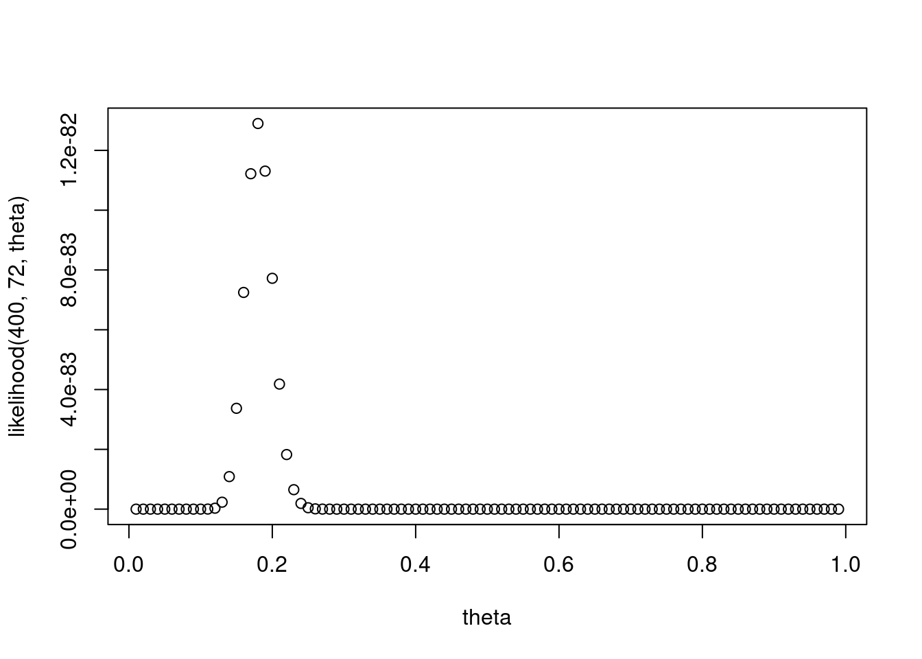
You can also do this with log likelihoods. This is typically more numerically stable to compute
loglike = function(n, y, theta) {
  return(y * log(theta) + (n - y) * log(1 - theta))
}
plot(theta, loglike(400, 72, theta))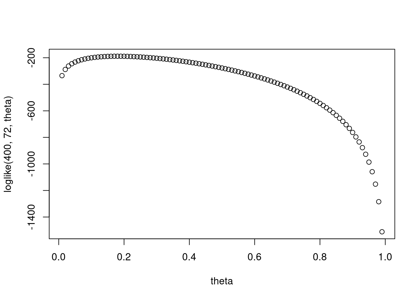
Having these plotted as points makes it difficult to see, let’s plot it as lines
plot(theta, loglike(400, 72, theta), type = "l")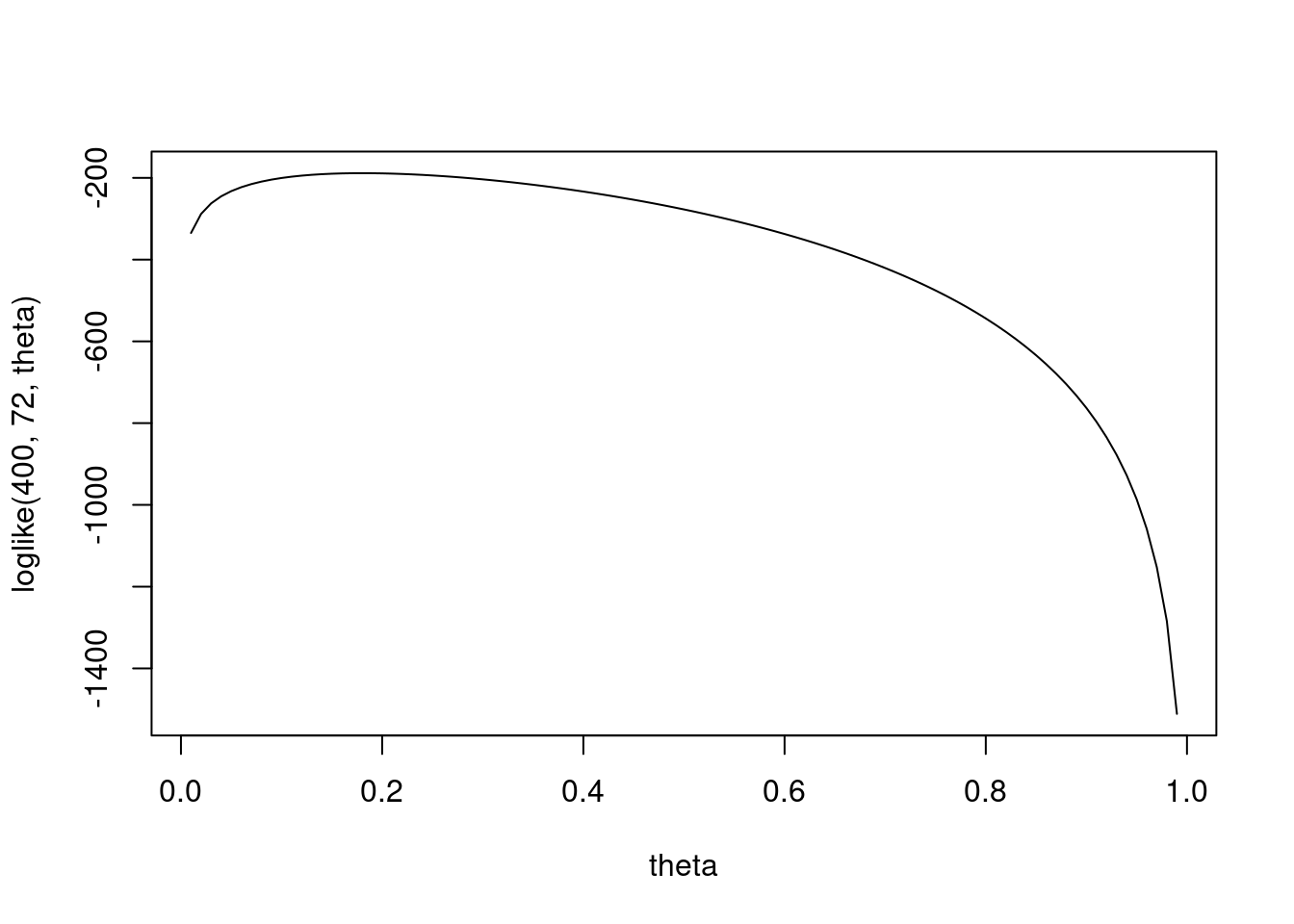
Each of the distributions introduced in Lesson 3 have convenient functions in R which allow you to evaluate the PDF/PMF, CDF, and quantile functions, as well as generate random samples from the distribution. To illustrate, see Table 11.1, which lists these functions for the normal distribution
| Function | What it does |
|---|---|
dnorm(x, mean, sd) |
Evaluate the PDF at x (mean = \mu and sd = \sqrt{\sigma^2}) |
pnorm(q, mean, sd) |
Evaluate the CDF at q |
qnorm(p, mean, sd) |
Evaluate the quantile function at p |
rnorm(n, mean, sd) |
Generate n pseudo-random samples from the normal distribution |
These four functions exist for each distribution where d... function evaluates the density/mass, p... evaluates the CDF, q... evaluates the quantile, and r... generates a sample. In Table 11.2 which lists the d... functions for some of the most popular distributions. The d can be replaced with p, q, or r for any of the distributions, depending on what you want to calculate.
For details enter ?dnorm to view R’s documentation page for the Normal distribution. As usual , replace the norm with any distribution to read the documentation for that distribution.
| Distribution | Function | Parameters |
|---|---|---|
| Binomial(n,p) | dbinom(x, size, prob) |
size = n, prob = p |
| Poisson(\lambda) | dpois(x, lambda) |
lambda = \lambda |
| Exp(\lambda) | dexp(x, rate) |
rate = \lambda |
| Gamma(\alpha, \beta) | dgamma(x, shape, rate) |
shape = \alpha, rate = \beta |
| Uniform(a, b) | dunif(x, min, max) |
min = a, max = b |
| Beta(\alpha, \beta) | dbeta(x, shape1, shape2) |
shape1 = \alpha, shape2 = \beta |
| N(\mu, \sigma^2) | dnorm(x, mean, sd) |
mean = \mu, sd = \sqrt{\sigma^2} |
| t_v | dt(x, df) |
df = v |