---
title : 'The EM algorithm for Mixture models - M2L3'
subtitle : 'Bayesian Statistics: Mixture Models'
categories:
- Bayesian Statistics
keywords:
- Mixture Models
- Maximum Likelihood Estimation
- Expectation-Maximization
- full data log likelihood
- EM algorithm
- E step
- M step
- notes
---
::: {.callout-note collapse="true"}
## TODO {.unnumbered .unlisted}
- [ ] In the EM algorithm generate animation from the outputs of the algorithm steps + prior & posterior
- [ ] Add example for carb data
:::
\index{mixture!EM algorithm}
\index{Maximum Likelihood Estimation}
**Maximum likelihood estimation** is the frequentist approach to estimate the parameters of statistical models. However, attempting to obtain maximum likelihood estimates (MLEs) $\hat{\omega}$ and $\hat{\theta}$ by directly maximizing the observed-data likelihood:
$$
\mathcal{L}(\omega,\theta) = \arg \max_{\omega,\theta}
\prod_{i=1}^{n} \sum_{k=1}^{K} \omega_k g_k(x_i|\theta_k)
$$ {#eq-mle-mixture-likelihood}
isn't feasible, as it is a non-convex optimization problem.
\index{optimization} \index{Newton-Raphson algorithm}
Using numerical optimization methods, such as the Newton-Raphson algorithm, can be challenging due when there are many components in the mixture.
It worthwhile mentioning that MLE is more of a **frequentist approach**, as it provides point estimates of the parameters rather than a distributional view. In contrast, Bayesian methods we will consider later provide a full posterior distribution of the parameters, which is more informative and allows for uncertainty quantification.
## EM algorithms for general mixtures :movie_camera: {#sec-EM-algorithm-for-general-mixtures}
{#fig-s_01 .column-margin width="53mm" group="slides"}
{#fig-s_02 .column-margin width="53mm" group="slides"}
{#fig-s_03 .column-margin width="53mm" group="slides"}
\index{EM algorithm} \index{Expectation-Maximization algorithm}
The **EM algorithm** comes up a lot in NLP and other fields so it is worthwhile to understand it the way we will do so in the course.
It also important that the EM algorithm we use for mixture models is from the 1970s and is not the same as the general EM algorithm. c.f. [@dempster1977maximum]
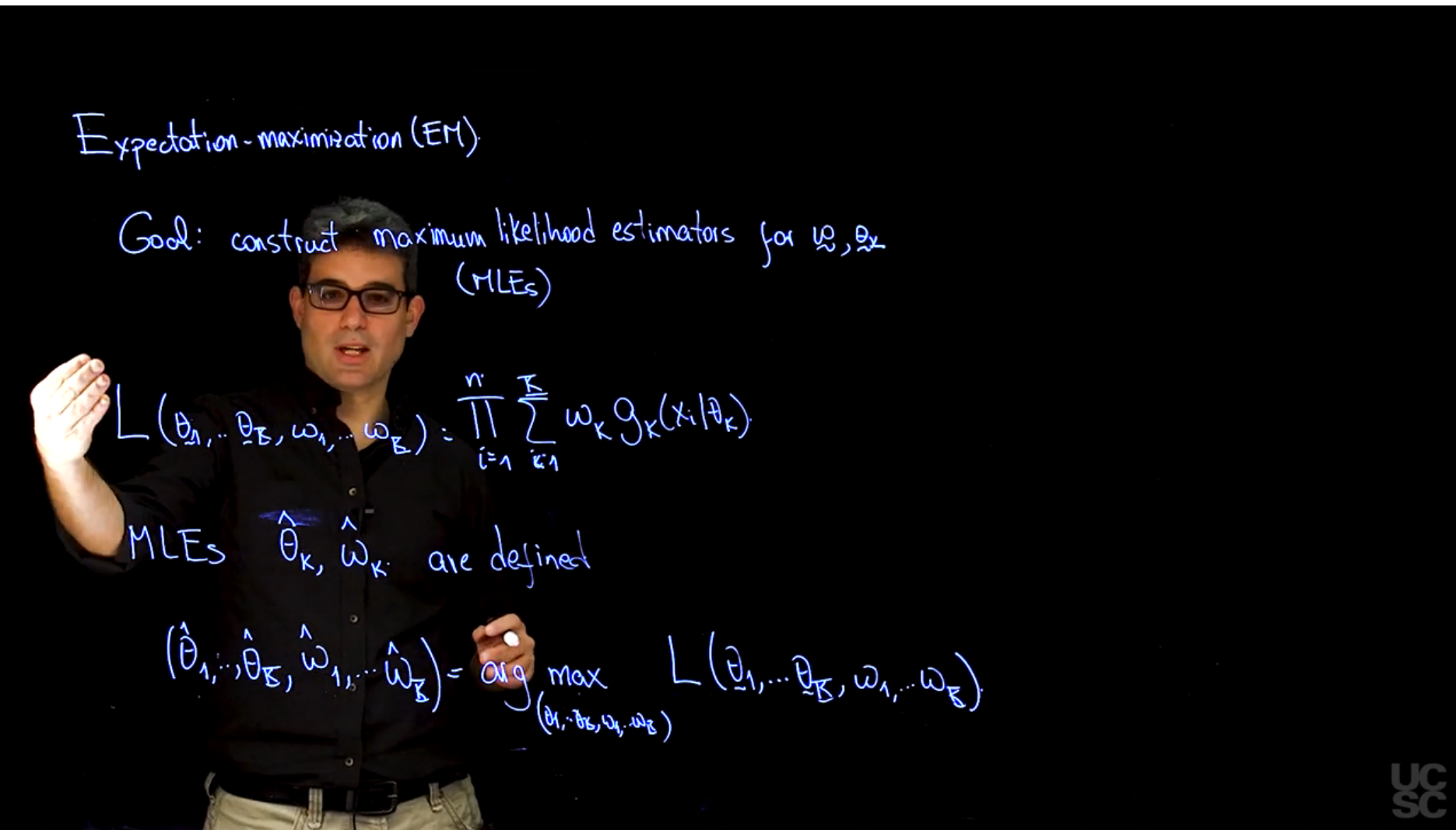
The goal of the EM algorithm is to find the parameters $\omega$ and $\theta$ for which the observed-data likelihood is maximized. We start with the **complete-data log-likelihood** Q function and then use it to construct maximum likelihood estimators for the parameters we are interested in, these are primarily the weights $\omega$ and the parameters $\theta$ of the distributional components.
we can express the complete-data log-likelihood as:
$$
L(\boldsymbol \theta,\boldsymbol \omega) = \prod_{i=1}^{N} \sum_{k=1}^{K} \omega_k g_k(x_i \mid \theta_k)
$$ {#eq-em-complete-data-log-likelihood}
MLE's $\hat{\theta}$ and $\hat{\omega}$ are defined
$$
(\boldsymbol \theta,\boldsymbol \omega) \stackrel{.}{=} \arg \max_{\boldsymbol \theta,\boldsymbol \omega} L(\boldsymbol \theta,\boldsymbol \omega)
$$
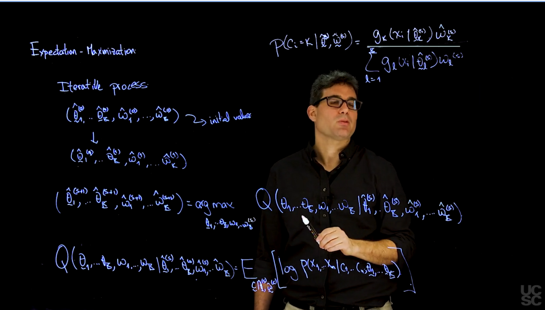
The EM algorithm is iterative and consists of two steps: the E-step and the M-step. The E-step computes the expected value of the complete-data log-likelihood given the observed data and the current parameter estimates, while the M-step maximizes this expected log-likelihood with respect to the parameters. However before we start these steps we need to set initial values for the parameters.
### E step:
Set
$$
Q(\omega,\theta \mid \omega^{(t)}, \theta^{(t)},x) = E_{c \mid \omega^{(t)},\theta^{(t)}, x} \left[ \log \mathbb{P}r(x,c \mid \omega,\theta) \right]
$$ {#eq-em-q-function}
Where $c$ is the latent variable indicating the component from which each observation was generated, $\omega$ are the weights, and $\theta$ are the parameters of the Gaussian components (means and standard deviations).
### M step:
Set
$$
\hat{\omega}^{(t+1)},\hat{\theta}^{(t+1)} = \arg \max_{\omega,\theta} Q(\omega,\theta \mid \hat{\omega}^{(t)}, \hat{\theta}^{(t)},y)
$$ {#eq-em-m-step}
where $\hat{\omega}^{(t)}$ and $\hat{\theta}^{(t)}$ are the current estimates of the parameters, and $y$ is the observed data.
These two steps are repeated until convergence, which is typically defined as the change in the full-data log-likelihood $Q$ function being below a certain threshold.
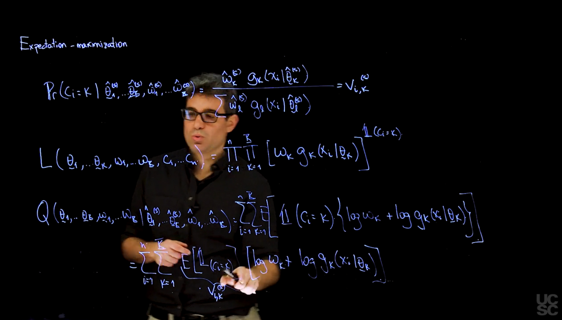
A key point is that if we condition each component independently on the $\omega, \theta, x$ we can write
$$
\mathbb{P}r(c_i=k \mid \omega, \theta, x_i) = \frac{\omega_k g_k(x_i \mid \theta_k)}{\sum_{j=1}^{K} \omega_j g_j(x_i \mid \theta_j)}= v_{ik}(\omega, \theta)
$$
where the value of $v_{ik}$ is interpreted as the probability that the $i$^-th^ observation comes from the $k$^-th^ component of the mixture assuming the population parameters $\omega$ and $\theta$.
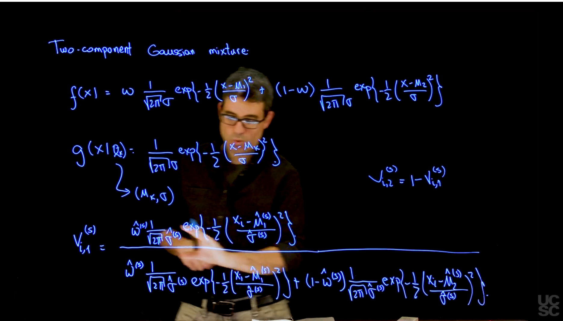
## EM for location Mixture of Gaussians :movie_camera: {#sec-em-for-location-mixtures-of-gaussians}
{#fig-s_04 .column-margin width="53mm" group="slides"}
{#fig-s_05 .column-margin width="53mm" group="slides"}
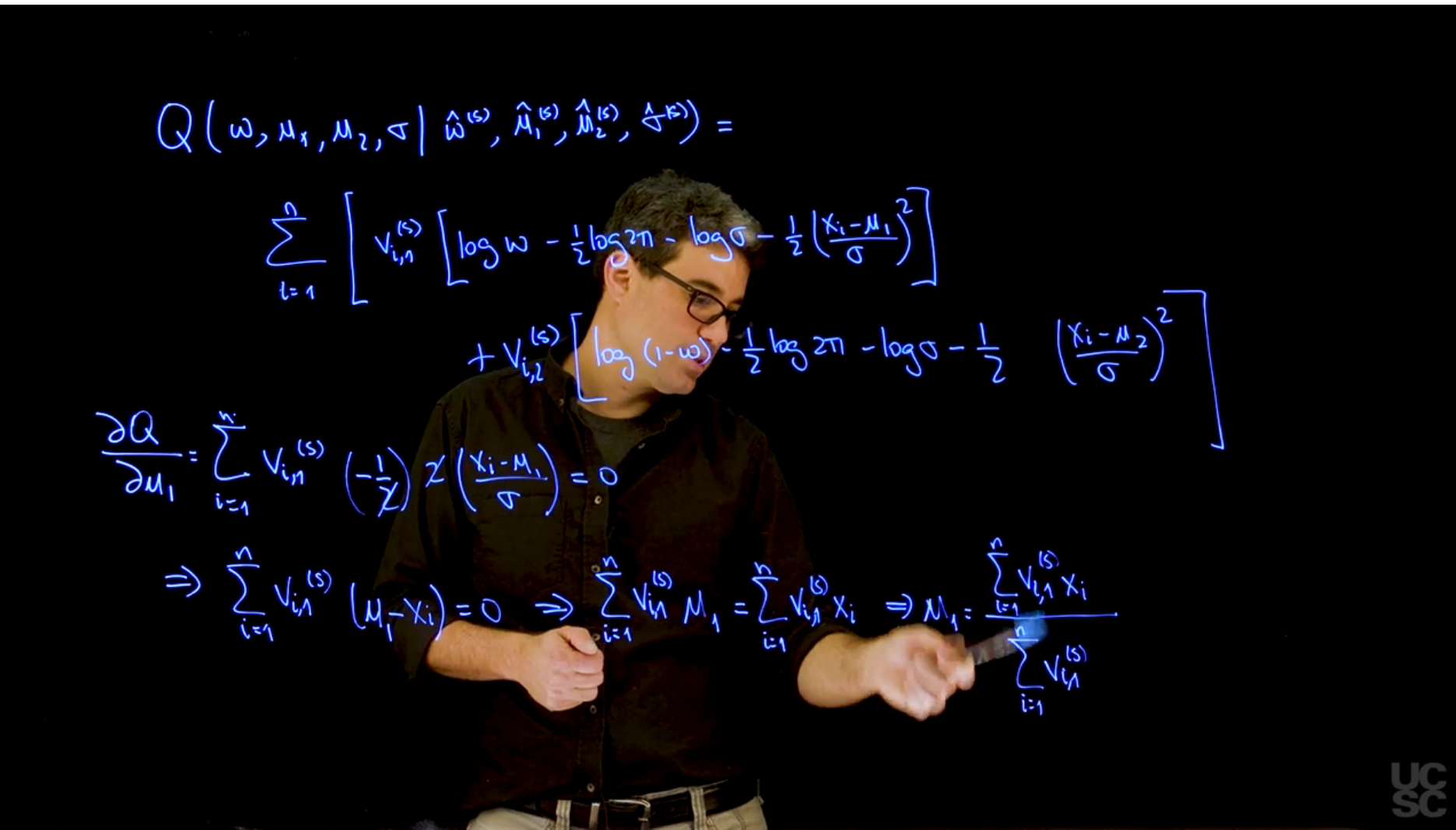{#fig-s_06 .column-margin width="53mm" group="slides"}
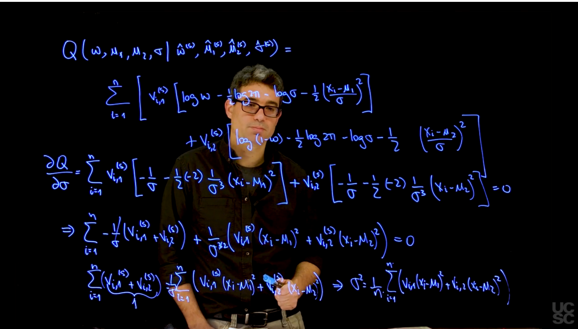{#fig-s_07 .column-margin width="53mm" group="slides"}
## EM example 1 :movie_camera: {#sec-em-example-1}
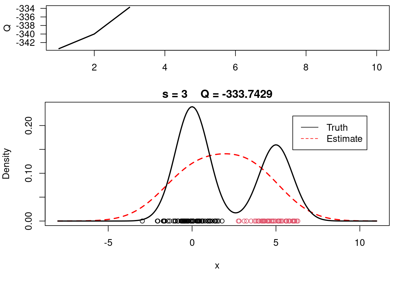
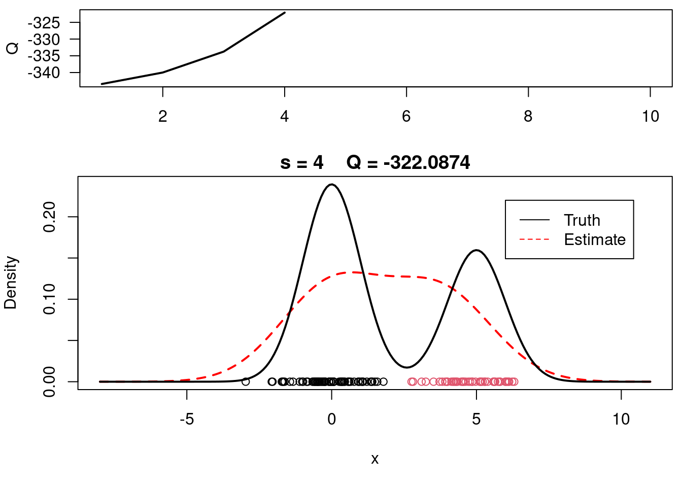
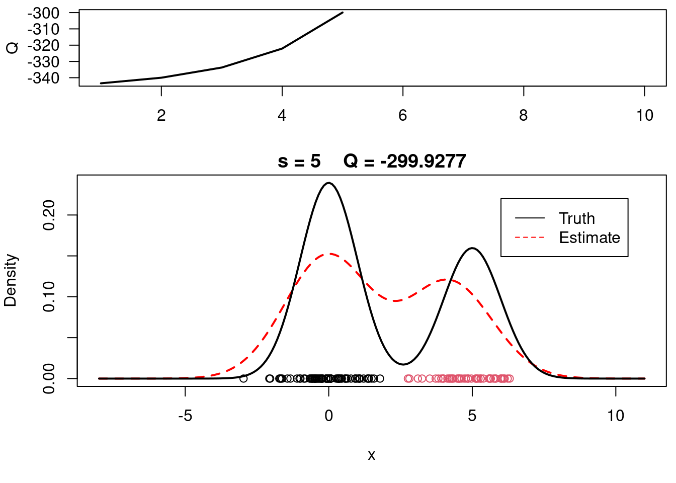
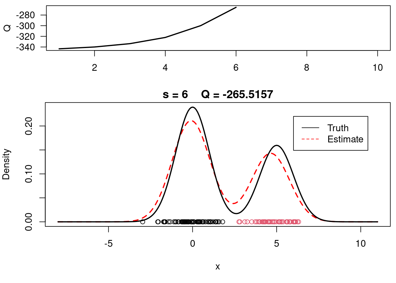
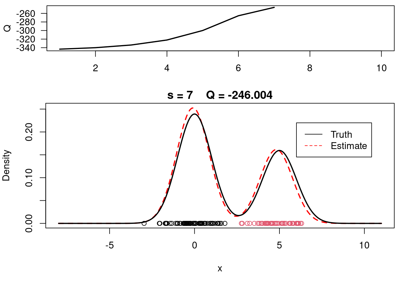
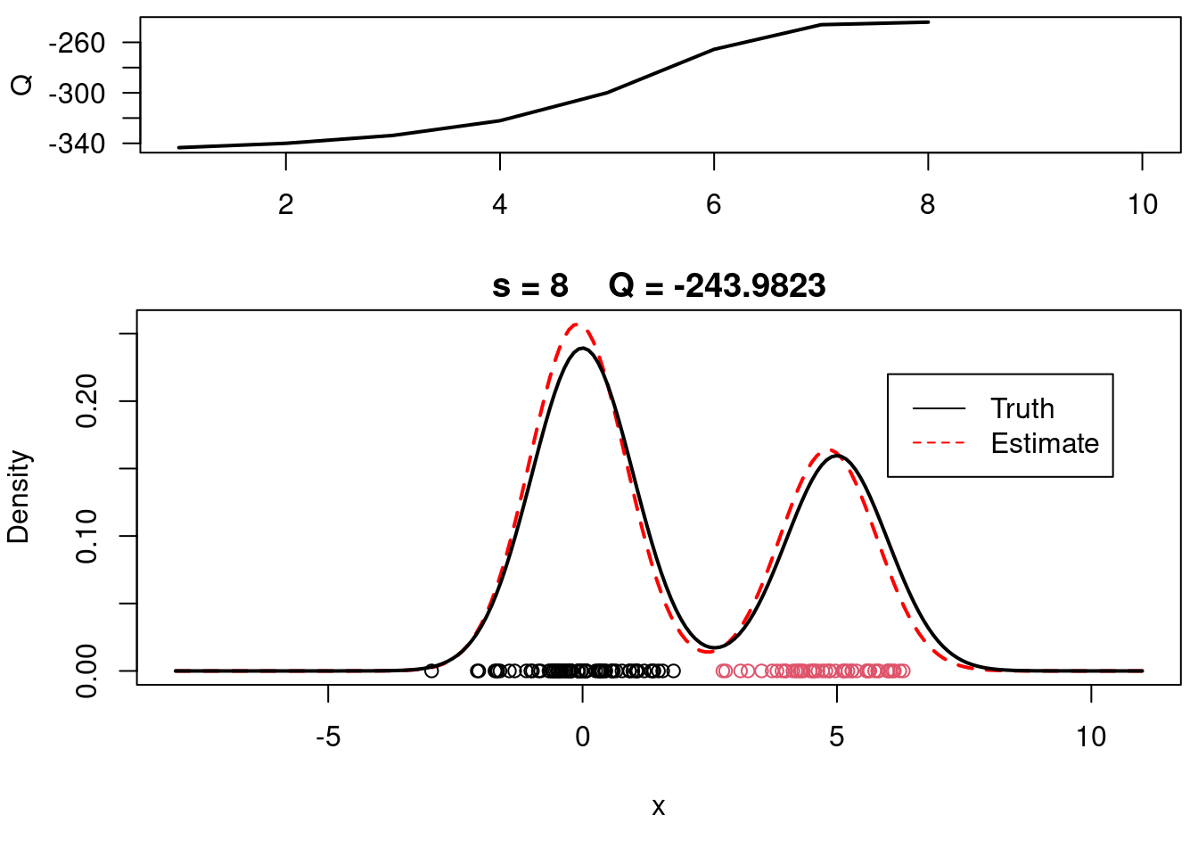
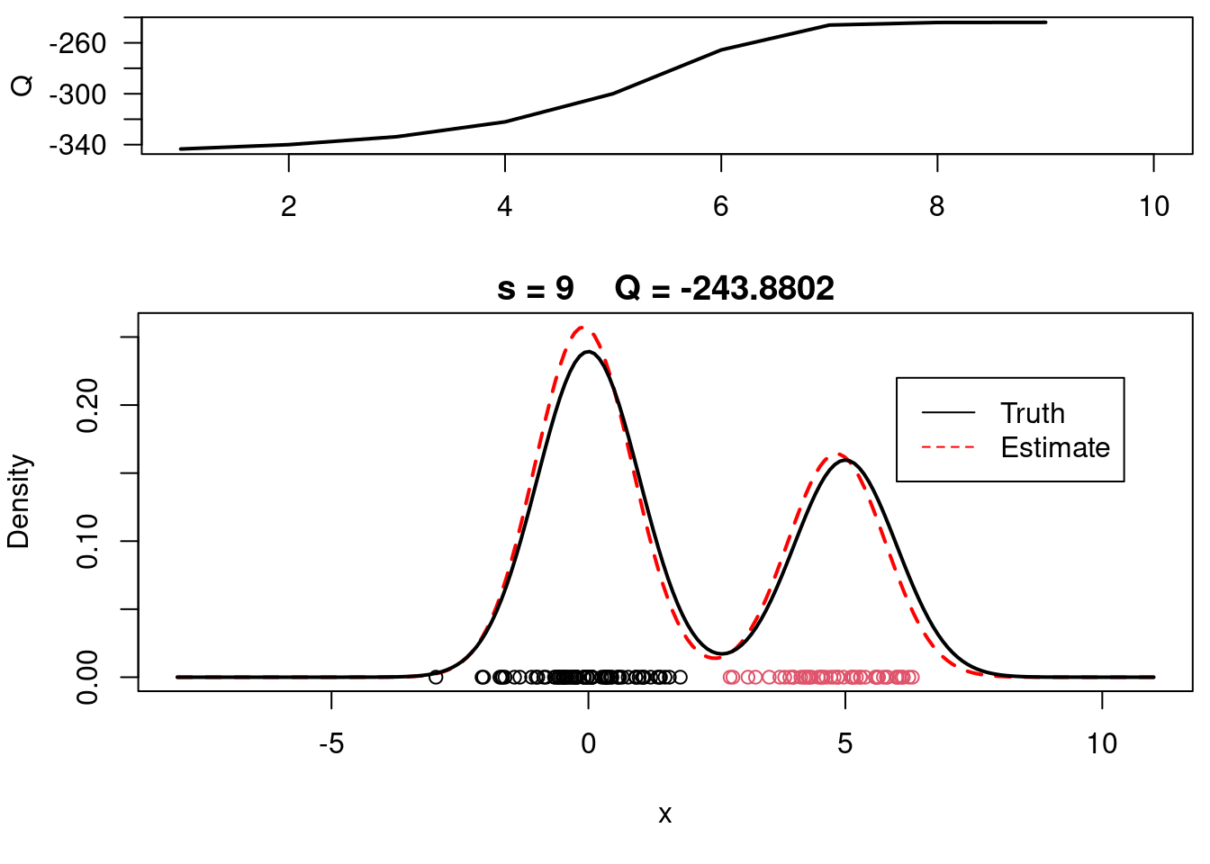
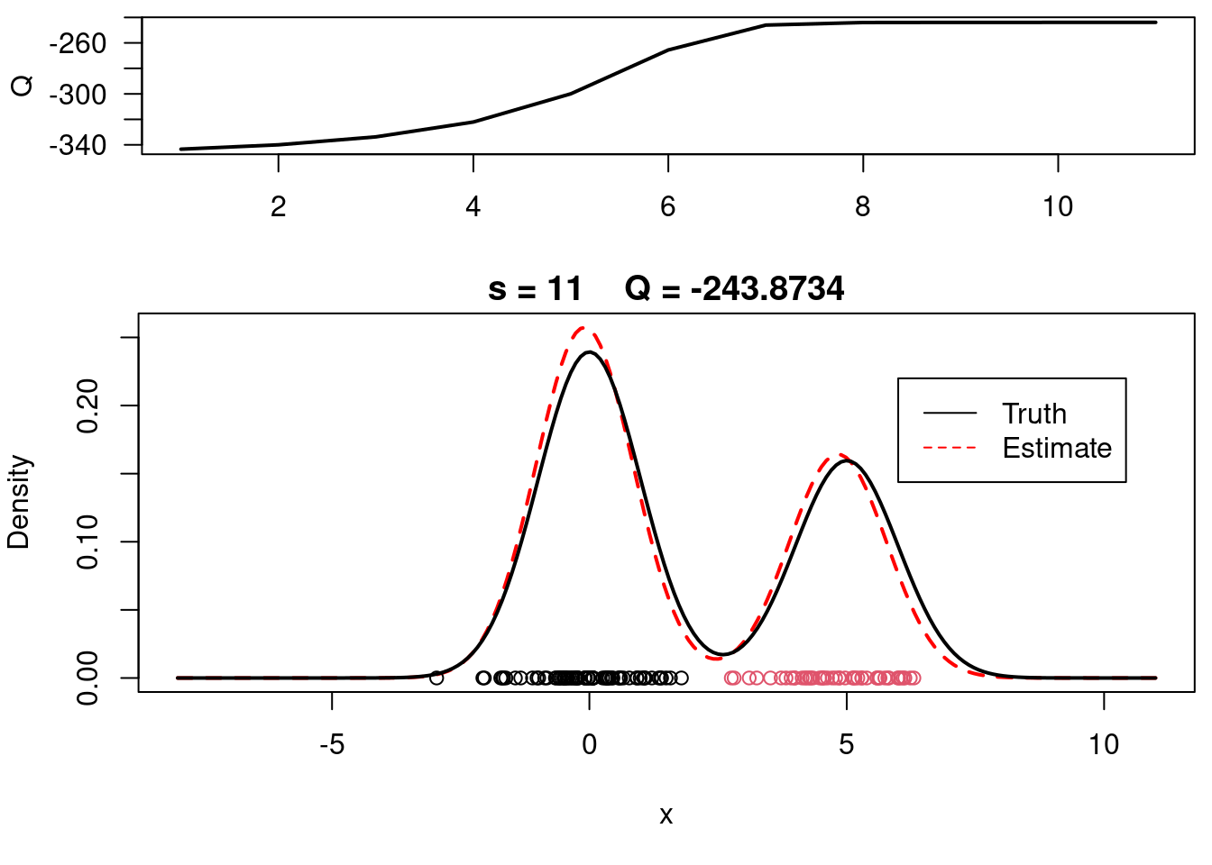
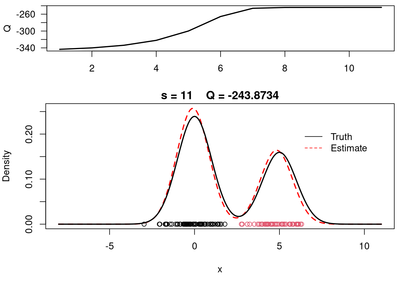
This video covers the code sample given in @lst-em-example-1 below. It is a simple implementation of the EM algorithm for fitting a 2-component Gaussian location mixture model to simulated data.
- This code sample is both cool and awkward.
- It is cool because it provides a step-by-step implementation of the EM algorithm, which is a fundamental concept in statistics and machine learning.
- It is not broken in to functions lacks useful variables naming which would reduce the amounts of comments and cognitive load.
- However it does provide nice visualizations of the EM algorithm in action - particularly if run inside of RStudio IDE (as shown in the video).
- would be interesting to make the number of components be drawn from a distribution rather than fixed at 2, then run the EM algorithm for multiple draws and pick the one with the best fit.
- Later on we learn about using *BIC* to select the number of components in a mixture model, which is a more principled approach than simply fixing the number of components at 2. However it stills seems that the number of components might be a RV even if it's prior would be centred at the *BIC estimate*.
## Sample code for EM example 1 :spiral_notepad: $\mathcal{R}$ {#sec-em-code-example-1}
```{r}
#| label: lst-em-example-1
#| lst-label: lst-em-example-1
#| lst-cap: "EM algorithm for fitting a 2-component Gaussian location mixture"
#### The algorithm is tested using simulated data
## Clear the environment and load required libraries
rm(list=ls())
set.seed(81196) # So that results are reproducible (same simulated data every time)
## Step 0 - Generate data from a mixture with 2 components:
## Ground Truth parameters initialization
KK = 2 # Number of components of the mixture
w.true = 0.6 # GT True weights associated with the components
mu.true = rep(0, KK) # initialize the true means list
mu.true[1] = 0 # GT mean for the first component
mu.true[2] = 5 # GT mean for the second component
sigma.true = 1 # GT standard deviation of all components
n = 120 # Number of synthetic samples to generate
# simulate the latent variables for the component indicator function
cc = sample(1:KK, n, replace=T, prob=c(w.true,1-w.true))
x = rep(0, n) # initialize the data vector x (or load data)
for(i in 1:n){ # for each observation
# sample from a distribution with mean selected by component indicator
# the SD is the same for all components as this is a location mixture
x[i] = rnorm(1, mu.true[cc[i]], sigma.true)
}
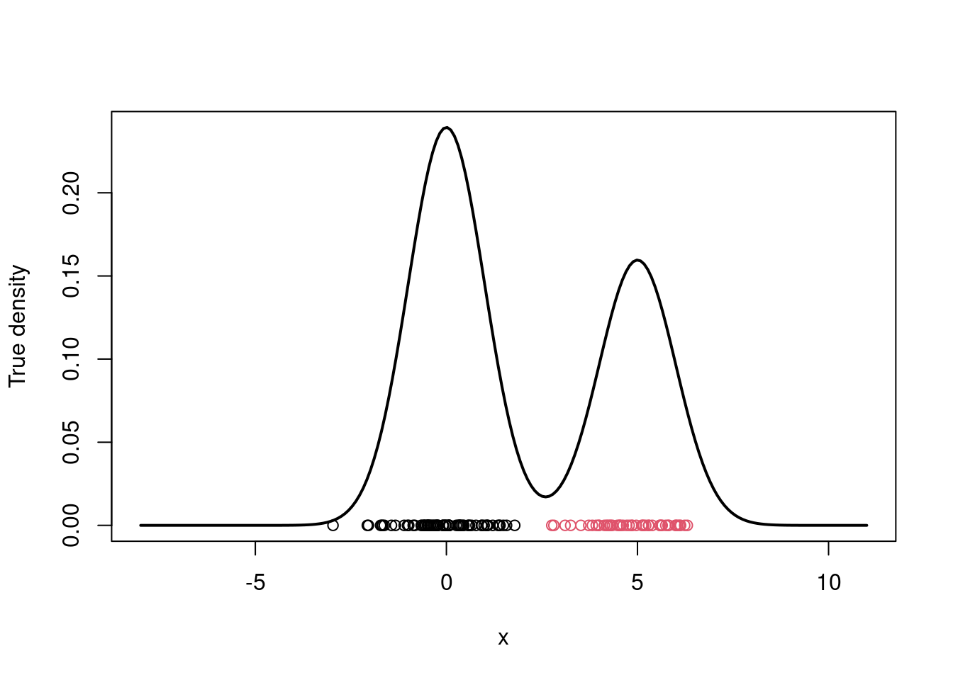
# Plot the true density
par(mfrow=c(1,1))
xx.true = seq(-8,11,length=200)
yy.true = w.true*dnorm(xx.true, mu.true[1], sigma.true) +
(1-w.true)*dnorm(xx.true, mu.true[2], sigma.true)
plot(xx.true, yy.true, type="l", xlab="x", ylab="True density", lwd=2)
points(x, rep(0,n), col=cc)
## Run the actual EM algorithm
## Initialize the parameters
w = 1/2 #Assign equal weight to each component to start with
mu = rnorm(KK, mean(x), sd(x)) #Random cluster centers randomly spread over the support of the data
sigma = sd(x) #Initial standard deviation
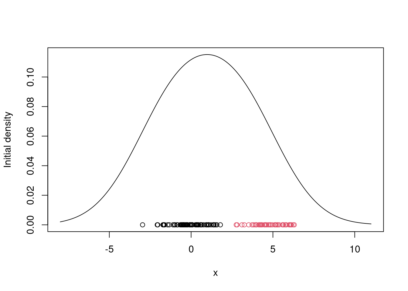
# Plot the initial guess for the density
xx = seq(-8,11,length=200)
yy = w*dnorm(xx, mu[1], sigma) + (1-w)*dnorm(xx, mu[2], sigma)
plot(xx, yy, type="l", ylim=c(0, max(yy)), xlab="x", ylab="Initial density")
points(x, rep(0,n), col=cc)
s = 0
sw = FALSE
QQ = -Inf
QQ.out = NULL
epsilon = 10^(-5)
##Checking convergence of the algorithm
while(!sw){
## E step
v = array(0, dim=c(n,KK))
v[,1] = log(w) + dnorm(x, mu[1], sigma, log=TRUE) #Compute the log of the weights
v[,2] = log(1-w) + dnorm(x, mu[2], sigma, log=TRUE) #Compute the log of the weights
for(i in 1:n){
v[i,] = exp(v[i,] - max(v[i,]))/sum(exp(v[i,] - max(v[i,]))) #Go from logs to actual weights in a numerically stable manner
}
## M step
# Weights
w = mean(v[,1])
mu = rep(0, KK)
for(k in 1:KK){
for(i in 1:n){
mu[k] = mu[k] + v[i,k]*x[i]
}
mu[k] = mu[k]/sum(v[,k])
}
# Standard deviations
sigma = 0
for(i in 1:n){
for(k in 1:KK){
sigma = sigma + v[i,k]*(x[i] - mu[k])^2
}
}
sigma = sqrt(sigma/sum(v))
##Check convergence
QQn = 0
for(i in 1:n){
QQn = QQn + v[i,1]*(log(w) + dnorm(x[i], mu[1], sigma, log=TRUE)) +
v[i,2]*(log(1-w) + dnorm(x[i], mu[2], sigma, log=TRUE))
}
if(abs(QQn-QQ)/abs(QQn)<epsilon){
sw=TRUE
}
QQ = QQn
QQ.out = c(QQ.out, QQ)
s = s + 1
print(paste(s, QQn))
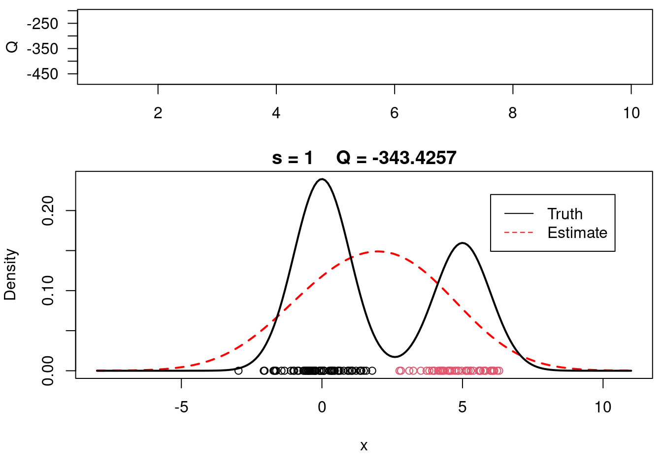
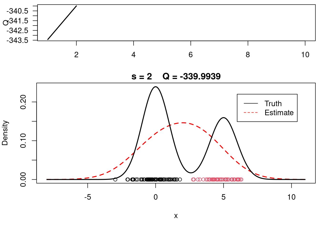
#Plot current estimate over data
layout(matrix(c(1,2),2,1), widths=c(1,1), heights=c(1.3,3))
par(mar=c(3.1,4.1,0.5,0.5))
plot(QQ.out[1:s],type="l", xlim=c(1,max(10,s)), las=1, ylab="Q", lwd=2)
par(mar=c(5,4,1.5,0.5))
xx = seq(-8,11,length=200)
yy = w*dnorm(xx, mu[1], sigma) + (1-w)*dnorm(xx, mu[2], sigma)
plot(xx, yy, type="l", ylim=c(0, max(c(yy,yy.true))), main=paste("s =",s," Q =", round(QQ.out[s],4)), lwd=2, col="red", lty=2, xlab="x", ylab="Density")
lines(xx.true, yy.true, lwd=2)
points(x, rep(0,n), col=cc)
legend(6,0.22,c("Truth","Estimate"),col=c("black","red"), lty=c(1,2))
}
#Plot final estimate over data
layout(matrix(c(1,2),2,1), widths=c(1,1), heights=c(1.3,3))
par(mar=c(3.1,4.1,0.5,0.5))
plot(QQ.out[1:s],type="l", xlim=c(1,max(10,s)), las=1, ylab="Q", lwd=2)

par(mar=c(5,4,1.5,0.5))
xx = seq(-8,11,length=200)
yy = w*dnorm(xx, mu[1], sigma) + (1-w)*dnorm(xx, mu[2], sigma)
plot(xx, yy, type="l", ylim=c(0, max(c(yy,yy.true))), main=paste("s =",s,"   Q =", round(QQ.out[s],4)), lwd=2, col="red", lty=2, xlab="x", ylab="Density")
lines(xx.true, yy.true, lwd=2)
points(x, rep(0,n), col=cc)
legend(6,0.22,c("Truth","Estimate"),col=c("black","red"), lty=c(1,2), bty="n")
```
## EM example 2 :movie_camera: {#sec-em-example-2}
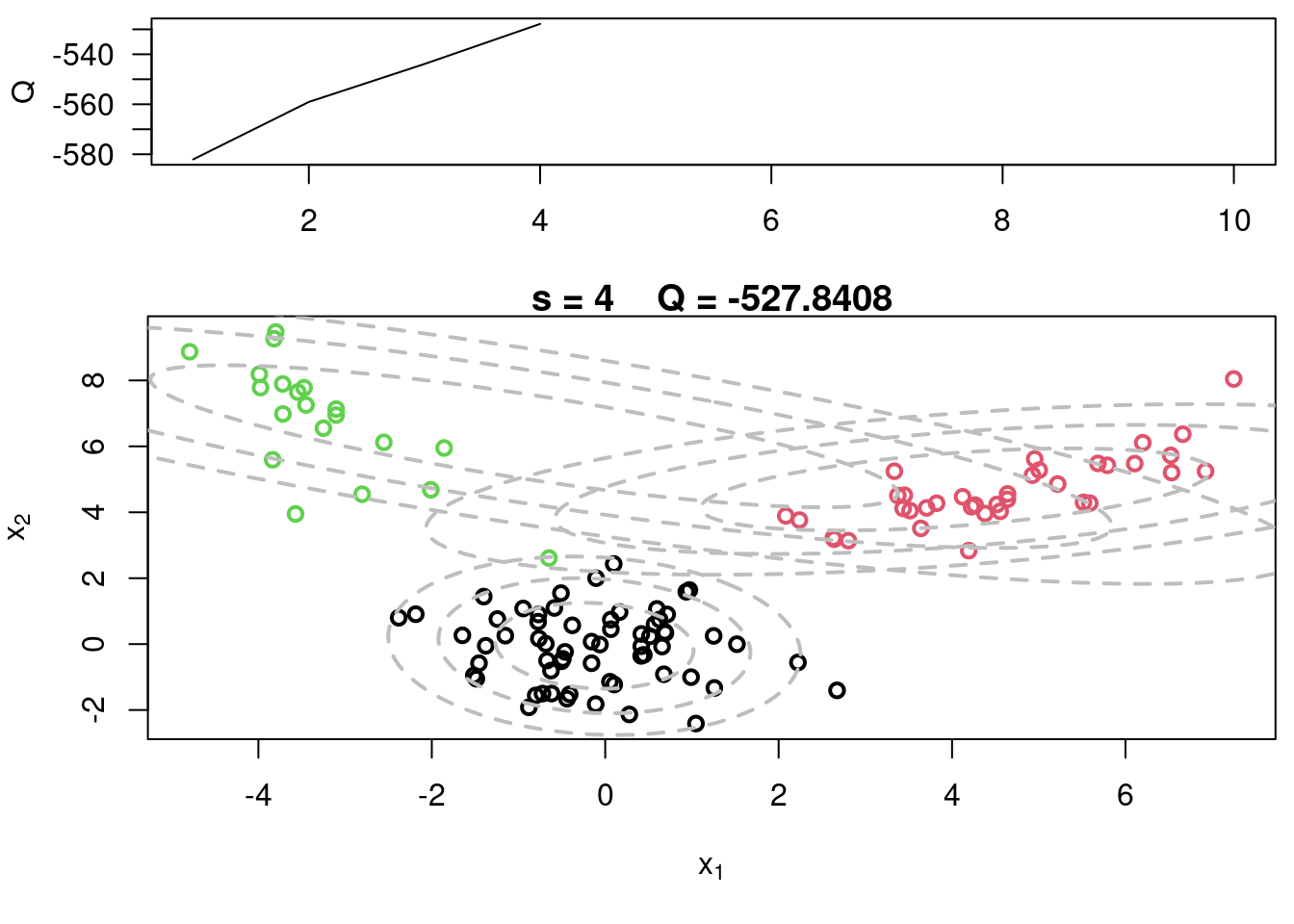
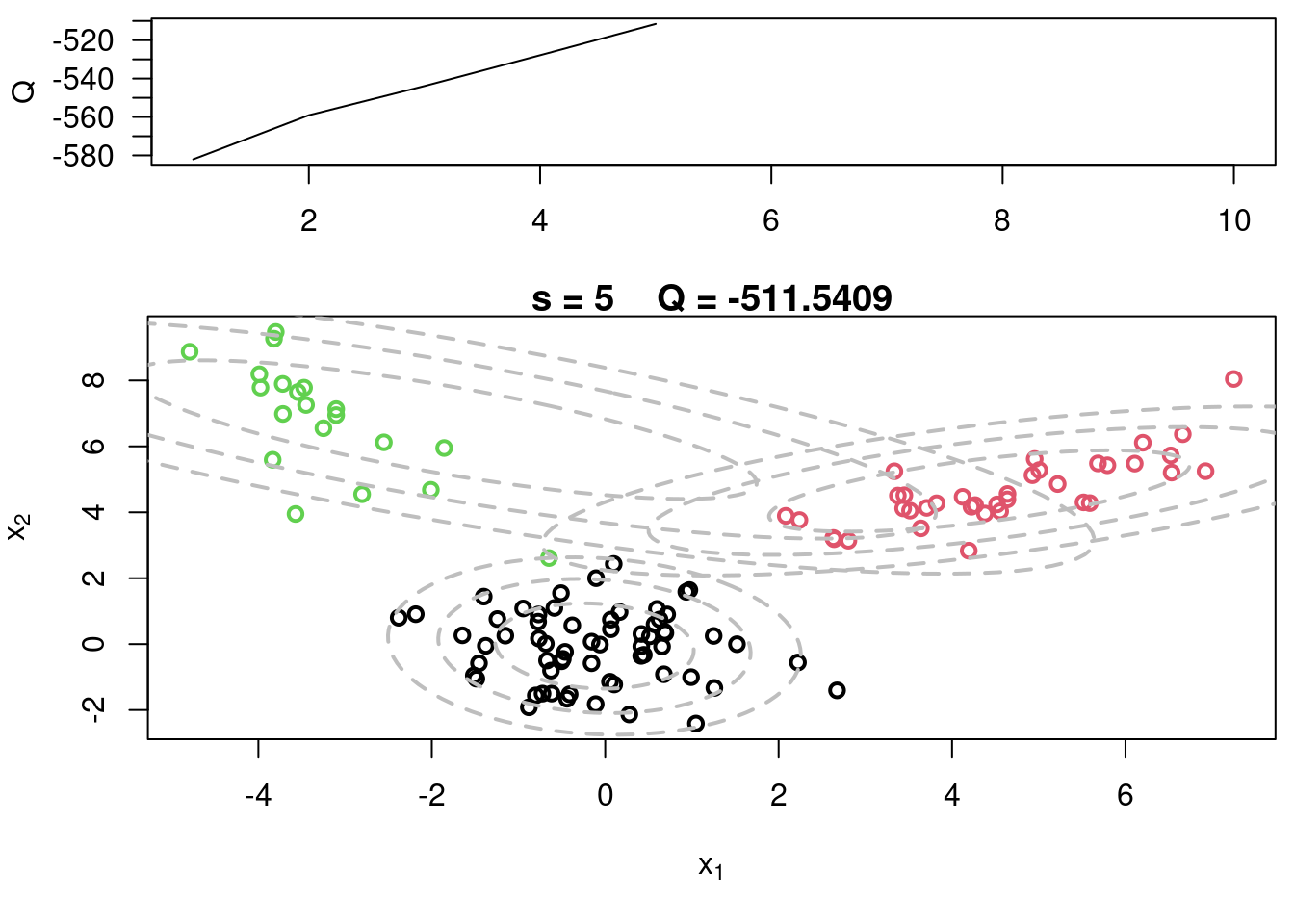
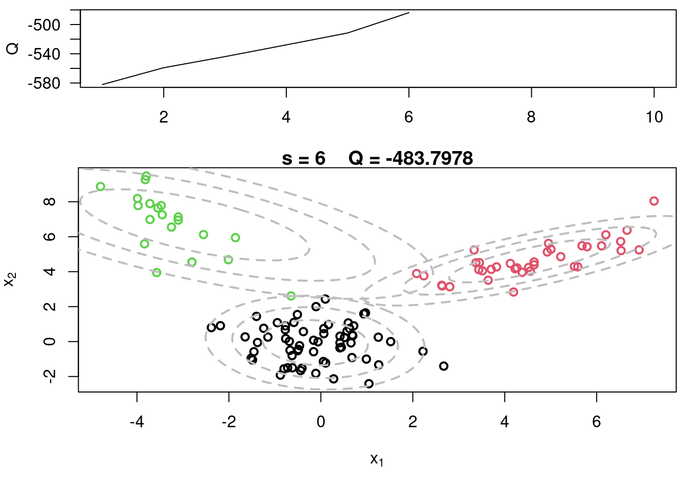
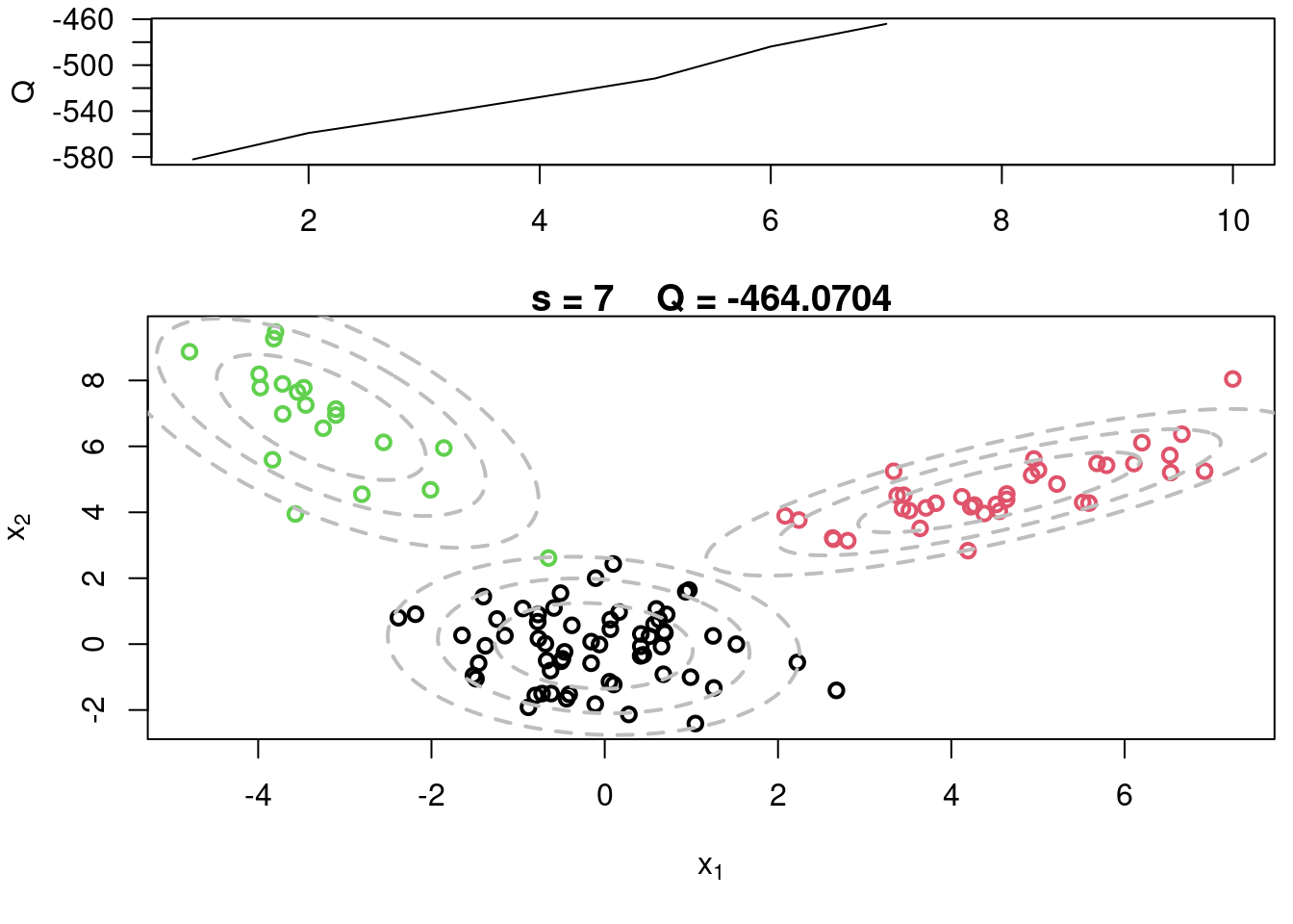
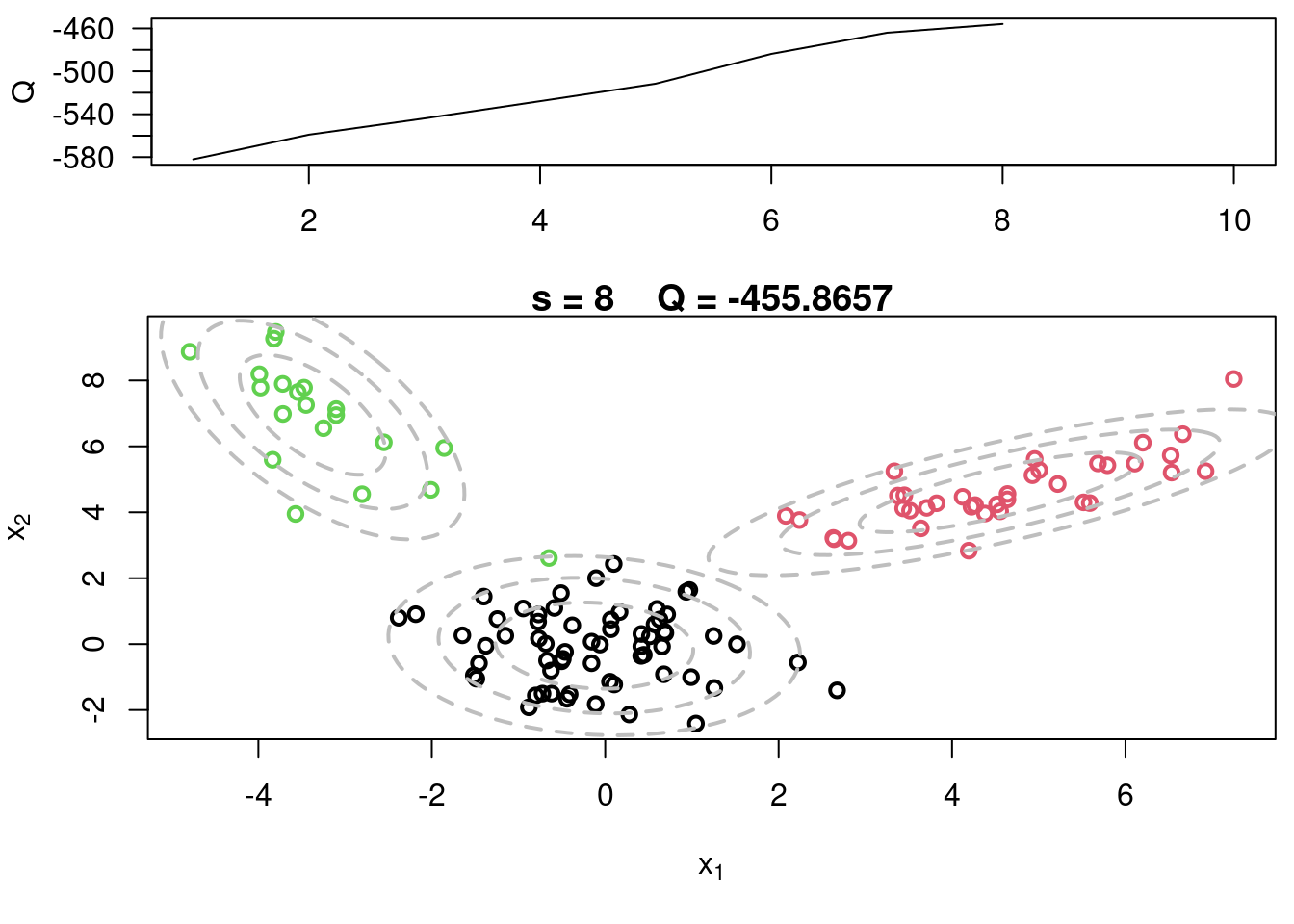
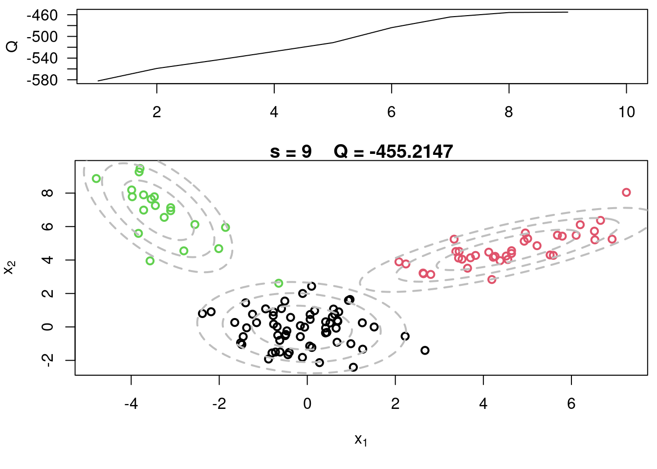
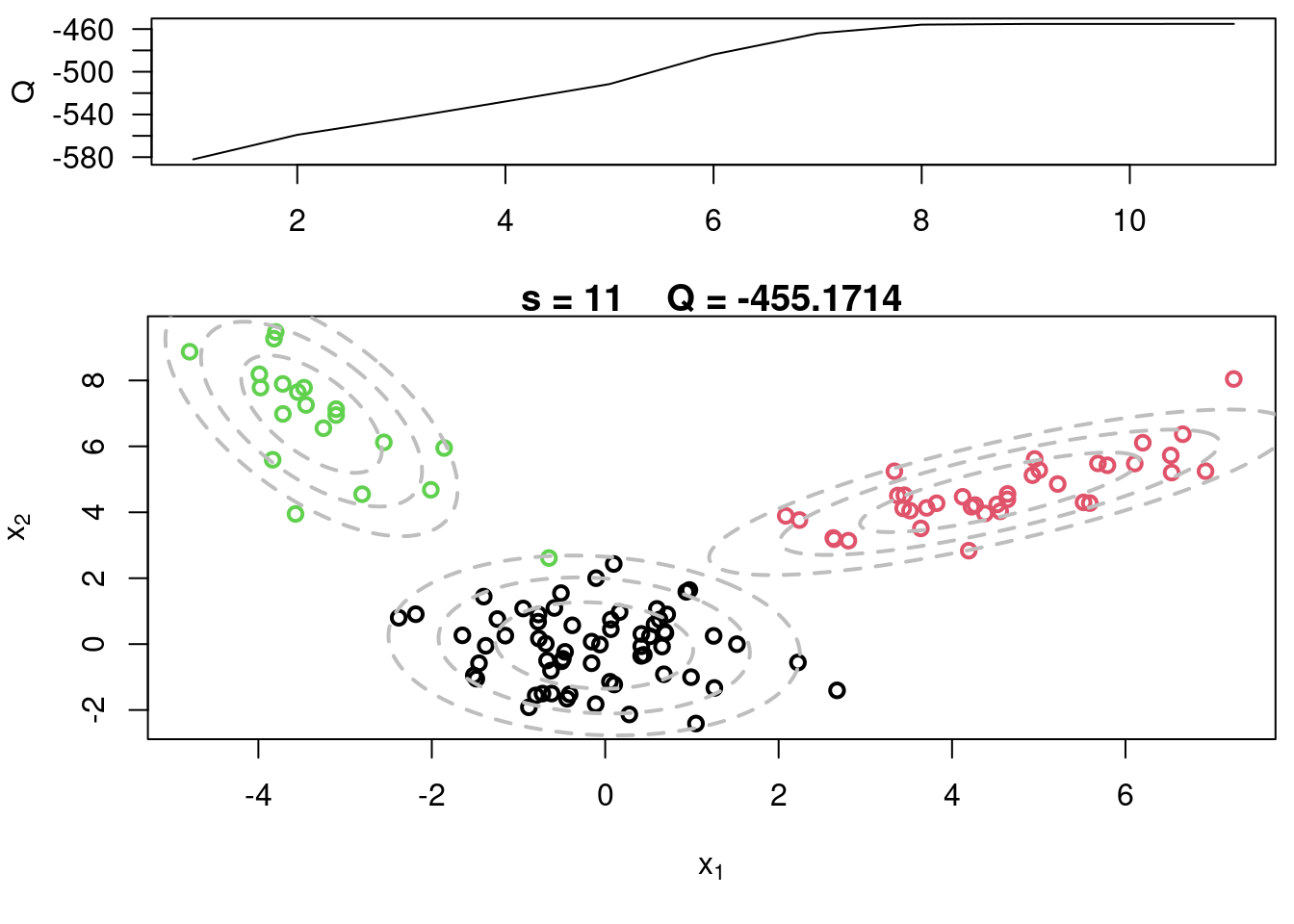
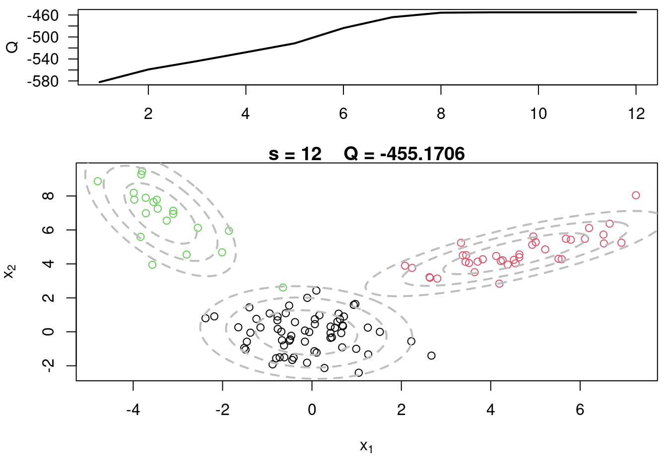
This video covers the code sample given in @sec-multivariate-EM below. It is a more advanced implementation of the EM algorithm for fitting a mixture of multivariate Gaussian components to simulated data.
## Sample code for multivariate normal EM :spiral_notepad: $\mathcal{R}$ {#sec-multivariate-EM}
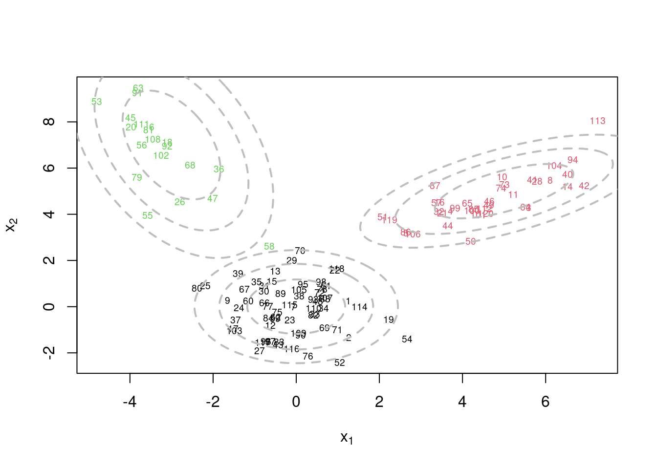
This variant differs from the code sample above in that it uses the `mvtnorm` package to generate **multivariate normal distributions**. It also uses the `ellipse` package to plot the ellipses around the means of the components.
```{r}
#| label: lst-em-example-2
#### Example of an EM algorithm for fitting a mixtures of K p-variate Gaussian components
#### The algorithm is tested using simulated data

## Clear the environment and load required libraries
rm(list=ls())
library(mvtnorm)    # Multivariate normals are not default in R
library(ellipse)    # Required for plotting
set.seed(63252)     # For reproducibility

## Generate data from a mixture with 3 components
KK      = 3
p       = 2
w.true = c(0.5,0.3,0.2)  # True weights associated with the components
mu.true     = array(0, dim=c(KK,p))
mu.true[1,] = c(0,0)   #True mean for the first component
mu.true[2,] = c(5,5)   #True mean for the second component
mu.true[3,] = c(-3,7)   #True mean for the third component
Sigma.true      = array(0, dim=c(KK,p,p))
Sigma.true[1,,] = matrix(c(1,0,0,1),p,p)   #True variance for the first component
Sigma.true[2,,] = matrix(c(2,0.9,0.9,1),p,p)   #True variance for the second component
Sigma.true[3,,] = matrix(c(1,-0.9,-0.9,4),p,p)   #True variance for the third component
n  = 120
cc = sample(1:3, n, replace=T, prob=w.true)
x  = array(0, dim=c(n,p))
for(i in 1:n){
  x[i,] = rmvnorm(1, mu.true[cc[i],], Sigma.true[cc[i],,])
}

par(mfrow=c(1,1))
plot(x[,1], x[,2], col=cc, type="n", xlab=expression(x[1]), ylab=expression(x[2]))
text(x[,1], x[,2], seq(1,n), col=cc, cex=0.6)
for(k in 1:KK){
  lines(ellipse(x=Sigma.true[k,,], centre=mu.true[k,], level=0.50), col="grey", lty=2, lwd=2)
  lines(ellipse(x=Sigma.true[k,,], centre=mu.true[k,], level=0.82), col="grey", lty=2, lwd=2)
  lines(ellipse(x=Sigma.true[k,,], centre=mu.true[k,], level=0.95), col="grey", lty=2, lwd=2)
}
#title(main="Data + True Components")
### Run the EM algorithm
## Initialize the parameters
w = rep(1,KK)/KK #Assign equal weight to each component to start with
mu = rmvnorm(KK, apply(x,2,mean), var(x)) #RandomCluster centers randomly spread over the support of the data
Sigma = array(0, dim=c(KK,p,p)) #Initial variances are assumed to be the same
Sigma[1,,] = var(x)/KK
Sigma[2,,] = var(x)/KK
Sigma[3,,] = var(x)/KK
par(mfrow=c(1,1))
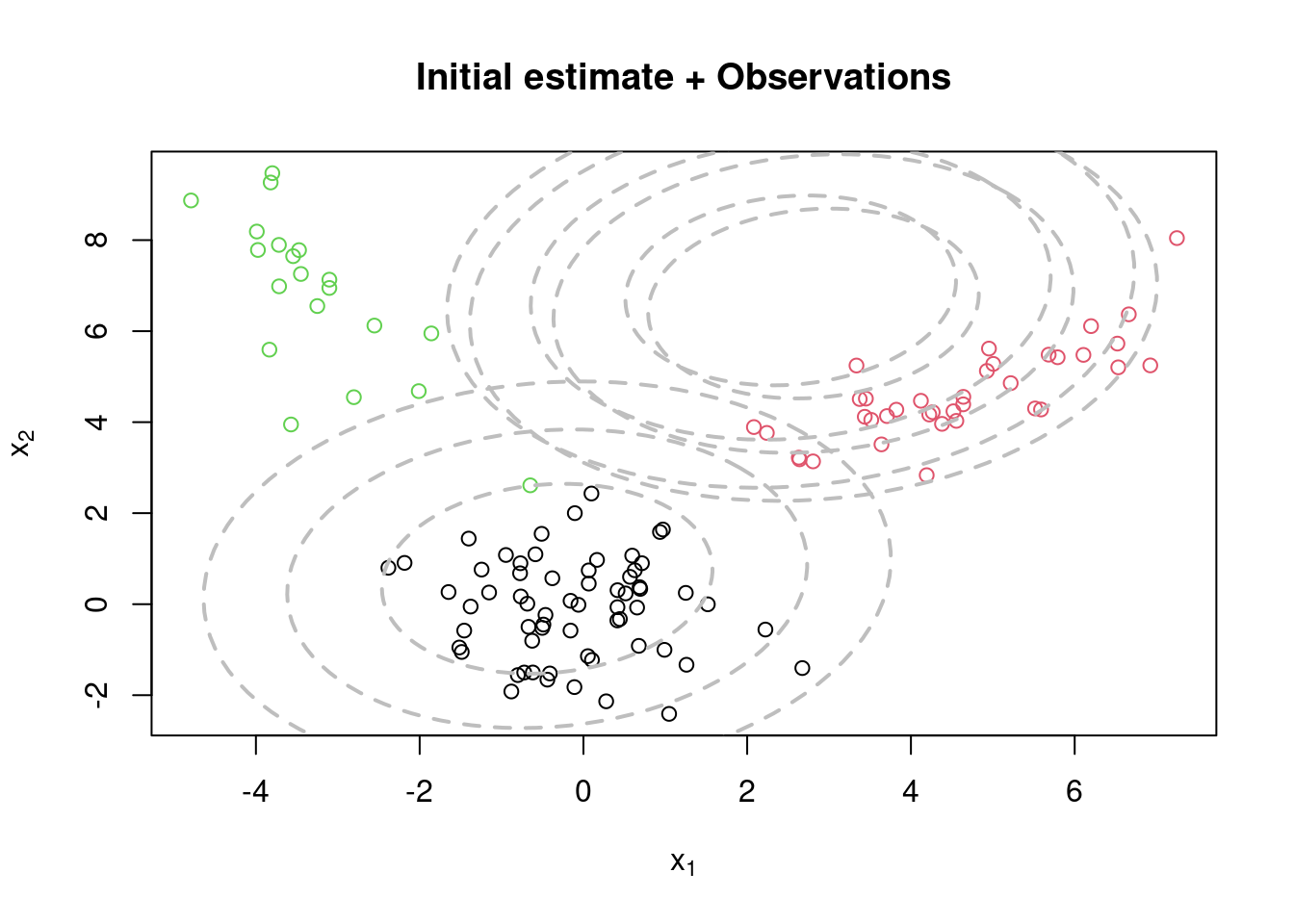
plot(x[,1], x[,2], col=cc, xlab=expression(x[1]), ylab=expression(x[2]))
for(k in 1:KK){
lines(ellipse(x=Sigma[k,,], centre=mu[k,], level=0.50), col="grey", lty=2, lwd=2)
lines(ellipse(x=Sigma[k,,], centre=mu[k,], level=0.82), col="grey", lty=2, lwd=2)
lines(ellipse(x=Sigma[k,,], centre=mu[k,], level=0.95), col="grey", lty=2, lwd=2)
}
title(main="Initial estimate + Observations")
s = 0
sw = FALSE
QQ = -Inf
QQ.out = NULL
epsilon = 10^(-5)
while(!sw){
## E step
v = array(0, dim=c(n,KK))
for(k in 1:KK){
v[,k] = log(w[k]) + dmvnorm(x, mu[k,], Sigma[k,,],log=TRUE) #Compute the log of the weights
}
for(i in 1:n){
v[i,] = exp(v[i,] - max(v[i,]))/sum(exp(v[i,] - max(v[i,]))) #Go from logs to actual weights in a numerically stable manner
}
## M step
w = apply(v,2,mean)
mu = array(0, dim=c(KK, p))
for(k in 1:KK){
for(i in 1:n){
mu[k,] = mu[k,] + v[i,k]*x[i,]
}
mu[k,] = mu[k,]/sum(v[,k])
}
Sigma = array(0, dim=c(KK, p, p))
for(k in 1:KK){
for(i in 1:n){
Sigma[k,,] = Sigma[k,,] + v[i,k]*(x[i,] - mu[k,])%*%t(x[i,] - mu[k,])
}
Sigma[k,,] = Sigma[k,,]/sum(v[,k])
}
##Check convergence
QQn = 0
for(i in 1:n){
for(k in 1:KK){
QQn = QQn + v[i,k]*(log(w[k]) + dmvnorm(x[i,],mu[k,],Sigma[k,,],log=TRUE))
}
}
if(abs(QQn-QQ)/abs(QQn)<epsilon){
sw=TRUE
}
QQ = QQn
QQ.out = c(QQ.out, QQ)
s = s + 1
print(paste(s, QQn))
#Plot current components over data
layout(matrix(c(1,2),2,1), widths=c(1,1), heights=c(1.3,3))
par(mar=c(3.1,4.1,0.5,0.5))
plot(QQ.out[1:s],type="l", xlim=c(1,max(10,s)), las=1, ylab="Q")
par(mar=c(5,4,1,0.5))
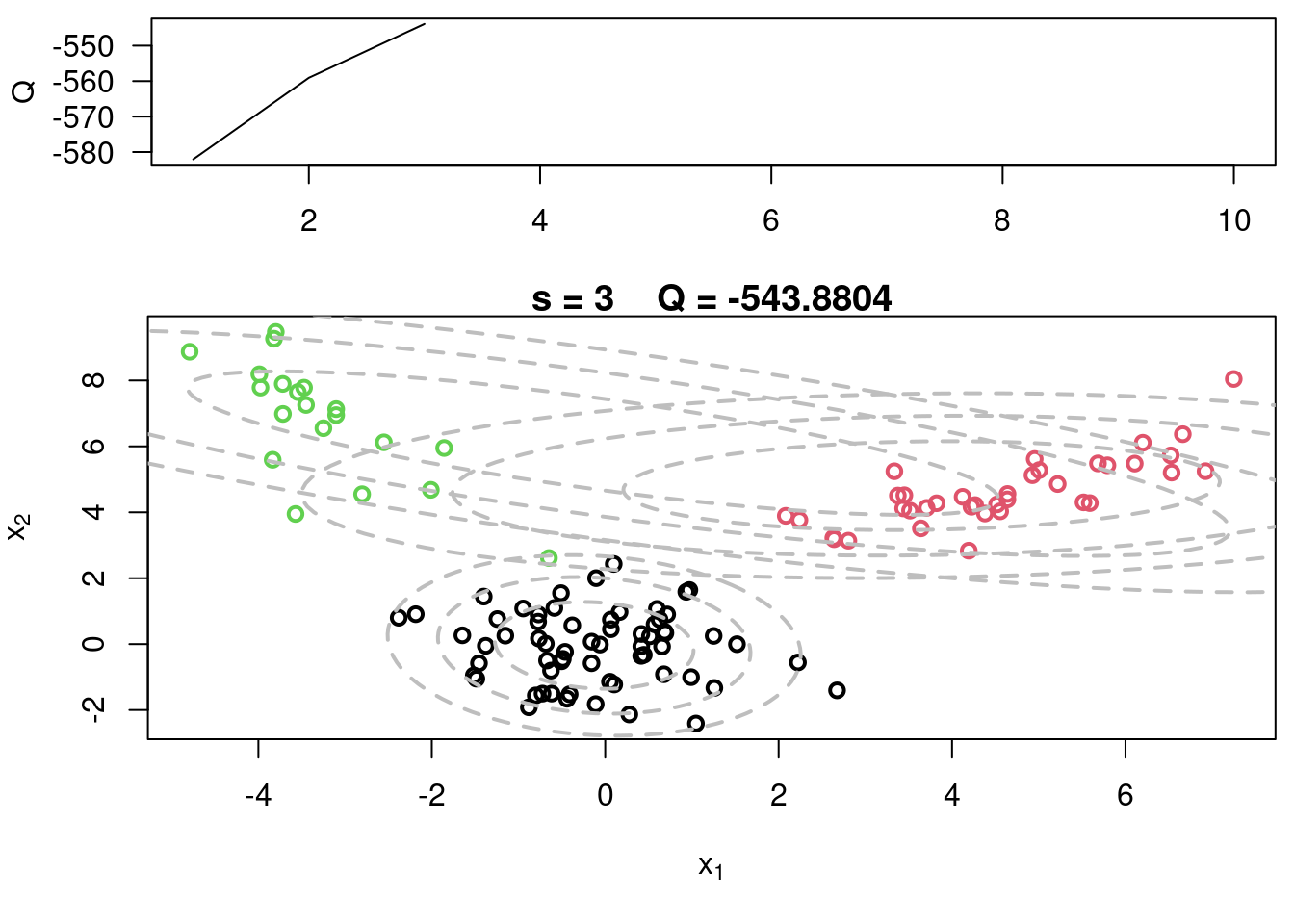
plot(x[,1], x[,2], col=cc, main=paste("s =",s," Q =", round(QQ.out[s],4)),
xlab=expression(x[1]), ylab=expression(x[2]), lwd=2)
for(k in 1:KK){
lines(ellipse(x=Sigma[k,,], centre=mu[k,], level=0.50), col="grey", lty=2, lwd=2)
lines(ellipse(x=Sigma[k,,], centre=mu[k,], level=0.82), col="grey", lty=2, lwd=2)
lines(ellipse(x=Sigma[k,,], centre=mu[k,], level=0.95), col="grey", lty=2, lwd=2)
}
}
#Plot current components over data
layout(matrix(c(1,2),2,1), widths=c(1,1), heights=c(1.3,3))
par(mar=c(3.1,4.1,0.5,0.5))
plot(QQ.out[1:s],type="l", xlim=c(1,max(10,s)), las=1, ylab="Q", lwd=2)

par(mar=c(5,4,1,0.5))
plot(x[,1], x[,2], col=cc, main=paste("s =",s,"   Q =", round(QQ.out[s],4)), xlab=expression(x[1]), ylab=expression(x[2]))
for(k in 1:KK){
  lines(ellipse(x=Sigma[k,,], centre=mu[k,], level=0.50), col="grey", lty=2, lwd=2)
  lines(ellipse(x=Sigma[k,,], centre=mu[k,], level=0.82), col="grey", lty=2, lwd=2)
  lines(ellipse(x=Sigma[k,,], centre=mu[k,], level=0.95), col="grey", lty=2, lwd=2)
}
```
## Mixture of Log Gaussians {#sec-mixture-of-log-gaussians}
::: {.callout-note collapse="true"}
## Prompt {.unnumbered .unlisted}
If your data had support on the positive real numbers rather than the whole real line, how could you use the EM algorithm you just learned to instead fit a mixture of log-Gaussian distributions? Would you need to recode your algorithm?
### Response {.unnumbered .unlisted}
Updating the algorithm is nontrivial - it requires derivatives for each parameter.
Depending on the distribution, we may need to add custom code to update each. We also need to update the distribution if these are changed.
So while the algorithm does not change, the code may change quite a bit.
:::
## Advanced EM algorithms {#sec-advanced-em-algorithms}
### HW: The EM for ZIP mixtures
Data on the lifetime (in years) of fuses produced by the ACME Corporation is available in the file `fuses.csv`:
Provide the EM algorithm to fit the mixture model
### HW+: The EM for Mixture Models