74 Clustering - M4L6

74.1 Mixture Models for Clustering 🎥

Figure 74.1: Clustering Mixture Models 1

Figure 74.2: Clustering Mixture Models 2

Figure 74.3: Clustering Mixture Models 3

Figure 74.4: Clustering Mixture Models 4

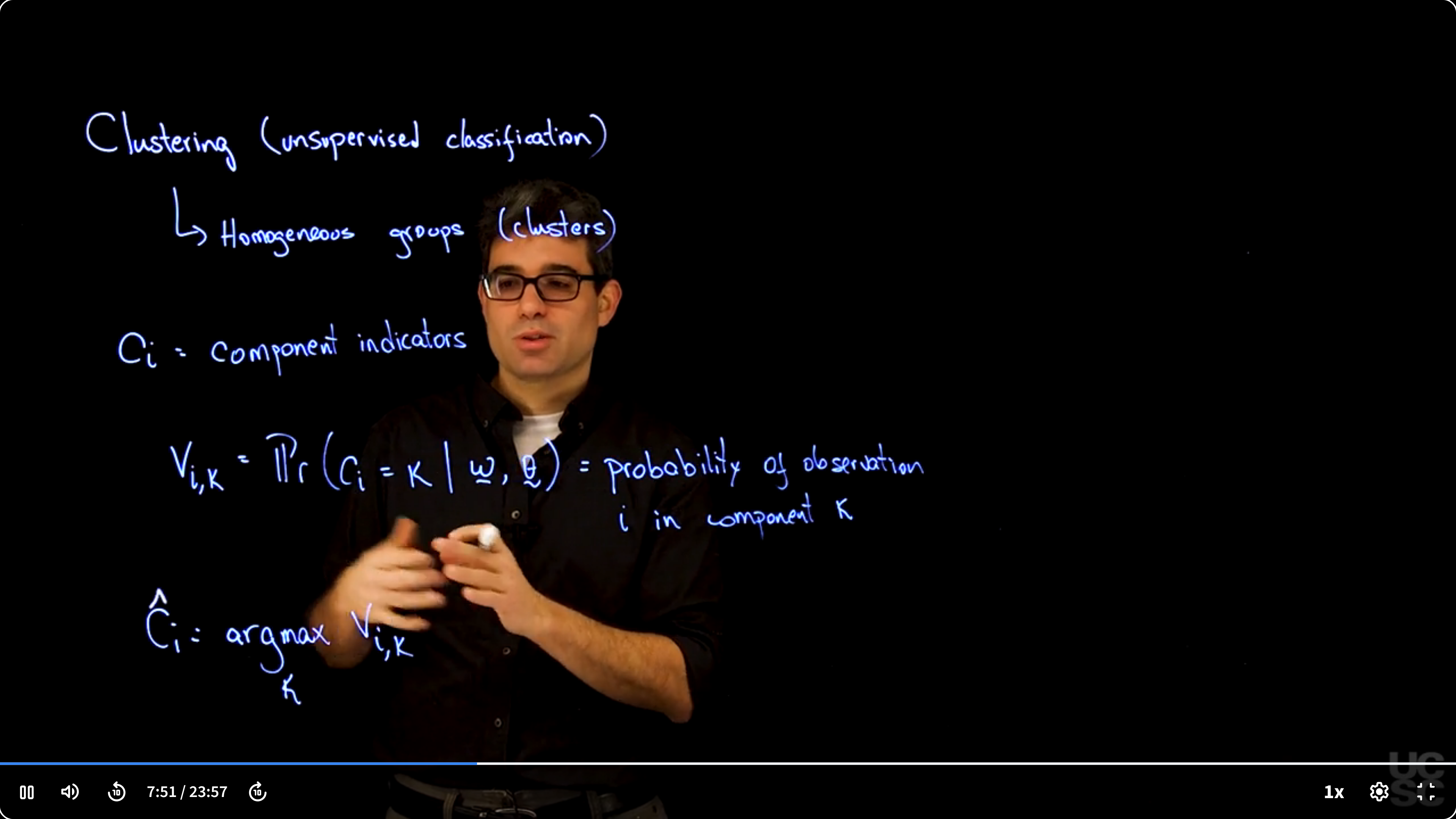
Clustering, aims to partition heterogeneous data into homogeneous groups (clusters). Common in biology and other domains, clustering helps identify underlying structure, such as species based on physiological features.

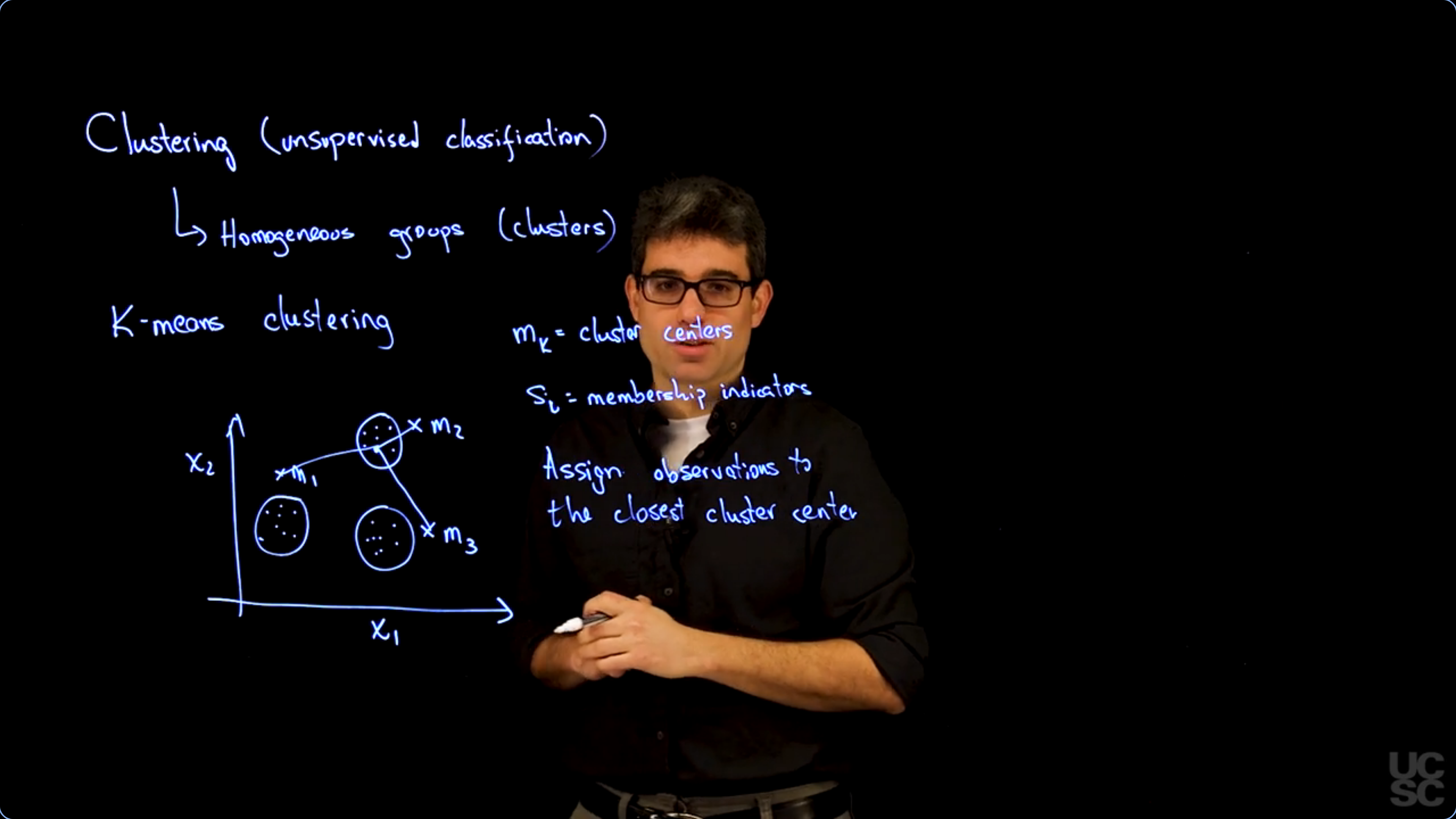
A widely-used method is K-means clustering, which:

• Fixes the number of clusters K

• Alternates between:

  1. Assignment step: Assigns each data point to its nearest cluster center.
  2. Update step: Recomputes centers as means of assigned points.

This process iterates until assignments stabilize.

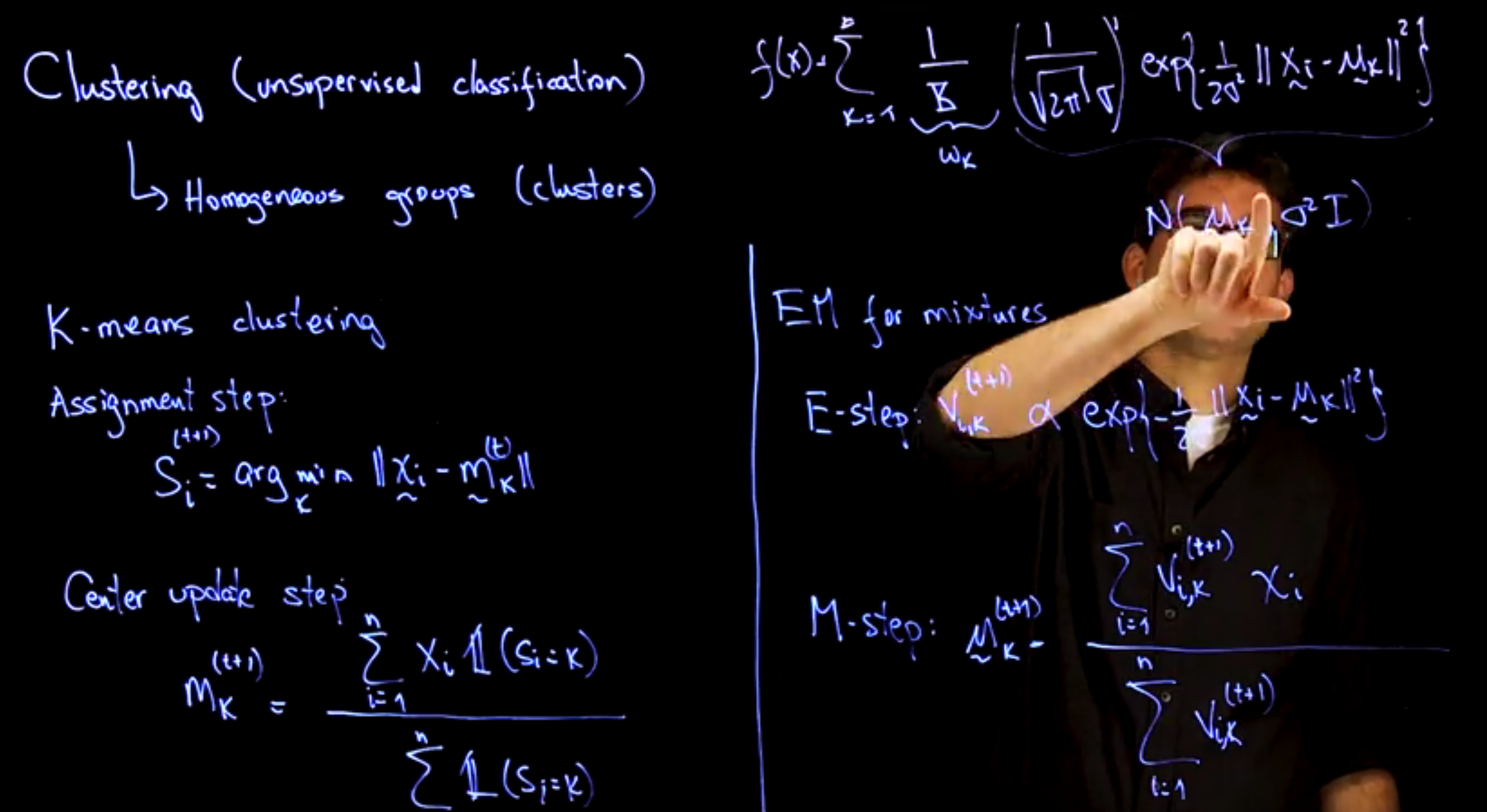
K-means is closely related to a mixture of Gaussians with:

• Equal component weights \omega_k = 1/K

• Shared spherical covariance \Sigma_k = \sigma^2 I

• Fitted via the EM algorithm, where:

  • E-step: compute soft assignment probabilities V_{ik}
  • M-step: update cluster means using weighted averages

If components are well-separated, EM approximates hard assignments similar to K-means.

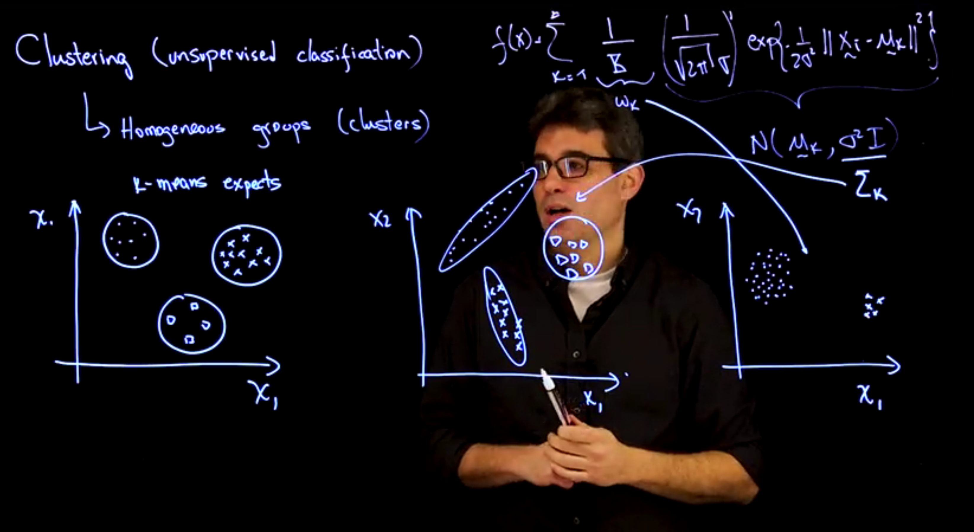
74.1.1 Limitations of K-means:

• Assumes equal-sized spherical clusters

• Fails with:

  • Correlated features
  • Different variances per dimension
  • Unequal cluster sizes

74.1.2 Advantages of Mixture Models:

• Allow flexible covariances \Sigma_k
• Estimate weights \omega_k
• Can use alternative kernels (e.g., t-distributions)
• Enable Bayesian clustering via MCMC

Thus, viewing K-means as a special case of Gaussian mixture models clarifies its assumptions and guides principled extensions.

74.2 Clustering example 🎥

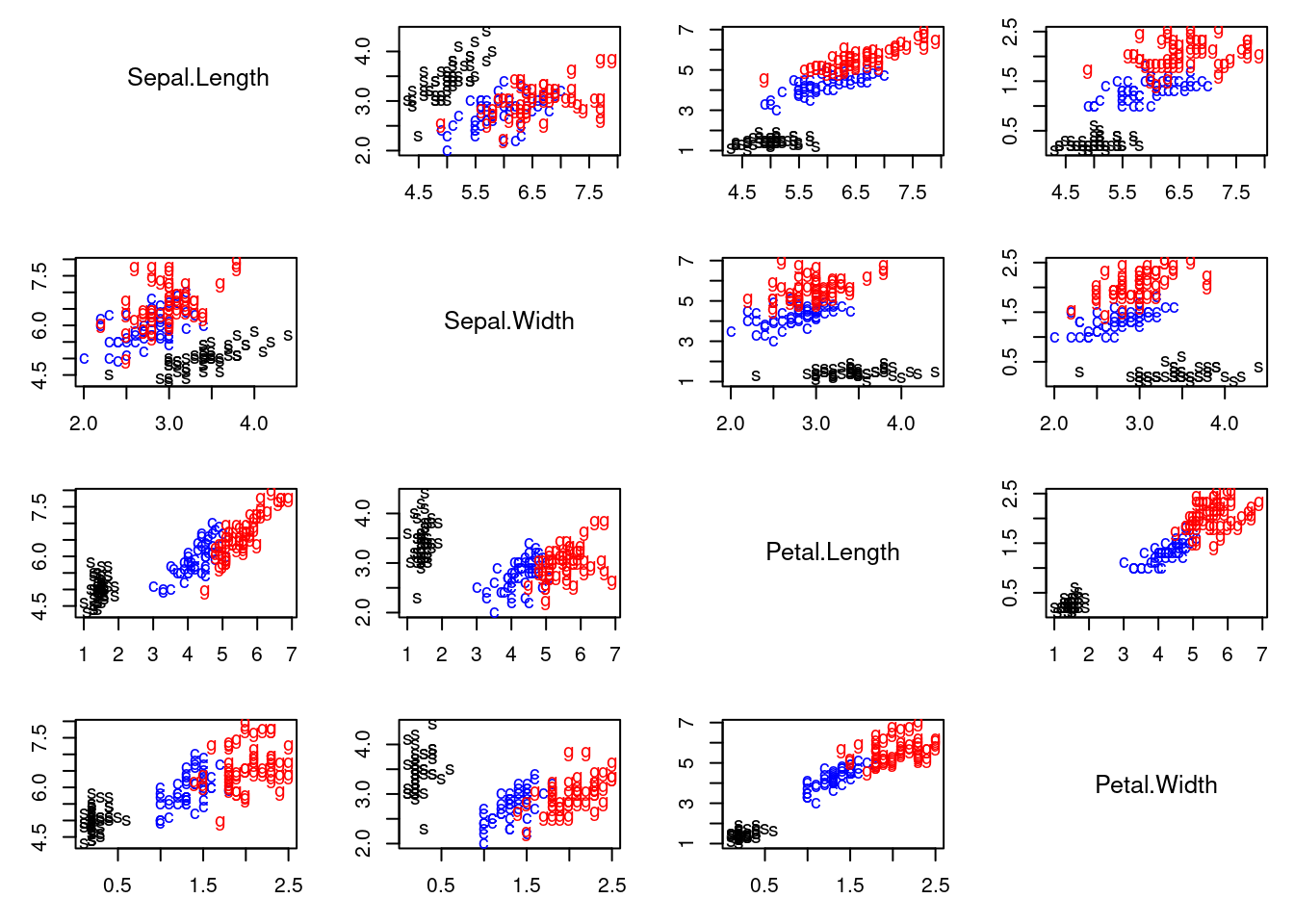
This video demonstrates clustering using the iris dataset, comparing K-means and a location and scale mixture model with K normals. It highlights how mixture models can flexibly adapt to data structure, unlike K-means’ rigid assumptions. The code is provided in

74.3 Clustering example 🗒️ \mathcal{R}

## Using mixture models for clustering in the iris dataset
## Compare k-means clustering and a location and scale mixture model with K normals

### Loading data and setting up global variables
rm(list=ls())
library(mclust)

Package 'mclust' version 6.1.1
Type 'citation("mclust")' for citing this R package in publications.

library(mvtnorm)

Attaching package: 'mvtnorm'

The following object is masked from 'package:mclust':

    dmvnorm

### Defining a custom function to create pair plots
### This is an alternative to the R function pairs() that allows for 
### more flexibility. In particular, it allows us to use text to label 
### the points
pairs2 = function(x, col="black", pch=16, labels=NULL, names = colnames(x)){
  n = dim(x)[1]
  p = dim(x)[2]
  par(mfrow=c(p,p))
  for(k in 1:p){
    for(l in 1:p){
      if(k!=l){
        par(mar=c(3,3,1,1)+0.1)
        plot(x[,k], x[,l], type="n", xlab="", ylab="")
        if(is.null(labels)){
          points(x[,k], x[,l], pch=pch, col=col)
        }else{
          text(x[,k], x[,l], labels=labels, col=col)
        }
      }else{
        plot(seq(0,5), seq(0,5), type="n", xlab="", ylab="", axes=FALSE)
        text(2.5,2.5,names[k], cex=1.2)
      }
    }
  }
}

## Setup data
data(iris)
x       = as.matrix(iris[,-5])
n       = dim(x)[1]
p       = dim(x)[2]       # Number of features
KK      = 3
epsilon = 0.0000001
par(mfrow=c(1,1))
par(mar=c(4,4,1,1))
colscale = c("black","blue","red")
shortnam  = c("s","c","g")
pairs2(x, col=colscale[iris[,5]], labels=shortnam[as.numeric(iris[,5])])


# Initialize the parameters of the algorithm
set.seed(63252)
numruns = 15
v.sum   = array(0, dim=c(numruns, n, KK))
QQ.sum  = rep(0, numruns)

for(ss in 1:numruns){
  w   = rep(1,KK)/KK  #Assign equal weight to each component to start with
  mu  = rmvnorm(KK, apply(x,2,mean), 3*var(x))   #Cluster centers randomly spread over the support of the data
  Sigma      = array(0, dim=c(KK,p,p))  #Initial variances are assumed to be the same
  Sigma[1,,] = var(x)
  Sigma[2,,] = var(x)
  Sigma[3,,] = var(x)
  
  sw     = FALSE
  QQ     = -Inf
  QQ.out = NULL
  s      = 0
  
  while(!sw){
    ## E step
    v = array(0, dim=c(n,KK))
    for(k in 1:KK){  #Compute the log of the weights
      v[,k] = log(w[k]) + mvtnorm::dmvnorm(x, mu[k,], Sigma[k,,], log=TRUE) 
    }
    for(i in 1:n){
      v[i,] = exp(v[i,] - max(v[i,]))/sum(exp(v[i,] - max(v[i,])))  #Go from logs to actual weights in a numerically stable manner
    }
    
    ## M step
    w = apply(v,2,mean)
    mu = matrix(0, nrow=KK, ncol=p)
    for(k in 1:KK){
      for(i in 1:n){
        mu[k,]    = mu[k,] + v[i,k]*x[i,]
      }
      mu[k,] = mu[k,]/sum(v[,k])
    }
    Sigma = array(0,dim=c(KK, p, p))
    for(k in 1:KK){
      for(i in 1:n){
        Sigma[k,,] = Sigma[k,,] + v[i,k]*(x[i,] - mu[k,])%*%t(x[i,] - mu[k,])
      }
      Sigma[k,,] = Sigma[k,,]/sum(v[,k])
    }
    
    ##Check convergence
    QQn = 0
    for(i in 1:n){
      for(k in 1:KK){
        QQn = QQn + v[i,k]*(log(w[k]) + mvtnorm::dmvnorm(x[i,],mu[k,],Sigma[k,,],log=TRUE))
      }
    }
    if(abs(QQn-QQ)/abs(QQn)<epsilon){
      sw=TRUE
    }
    QQ = QQn
    QQ.out = c(QQ.out, QQ)
    s = s + 1
  }
  
  v.sum[ss,,] = v
  QQ.sum[ss]  = QQ.out[s]
  print(paste("ss =", ss))
}

[1] "ss = 1"
[1] "ss = 2"
[1] "ss = 3"
[1] "ss = 4"
[1] "ss = 5"
[1] "ss = 6"
[1] "ss = 7"
[1] "ss = 8"
[1] "ss = 9"
[1] "ss = 10"
[1] "ss = 11"
[1] "ss = 12"
[1] "ss = 13"
[1] "ss = 14"
[1] "ss = 15"

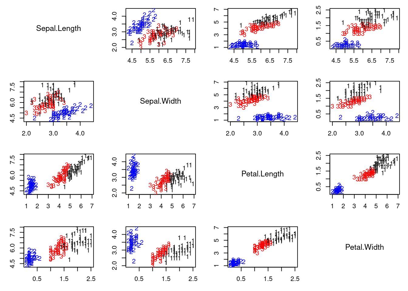
## Cluster reconstruction under the mixture model
cc = apply(v.sum[which.max(QQ.sum),,], 1 ,which.max)
colscale = c("black","blue","red")
pairs2(x, col=colscale[cc], labels=cc)
ARImle = adjustedRandIndex(cc, as.numeric(iris[,5]))  # Higher values indicate larger agreement

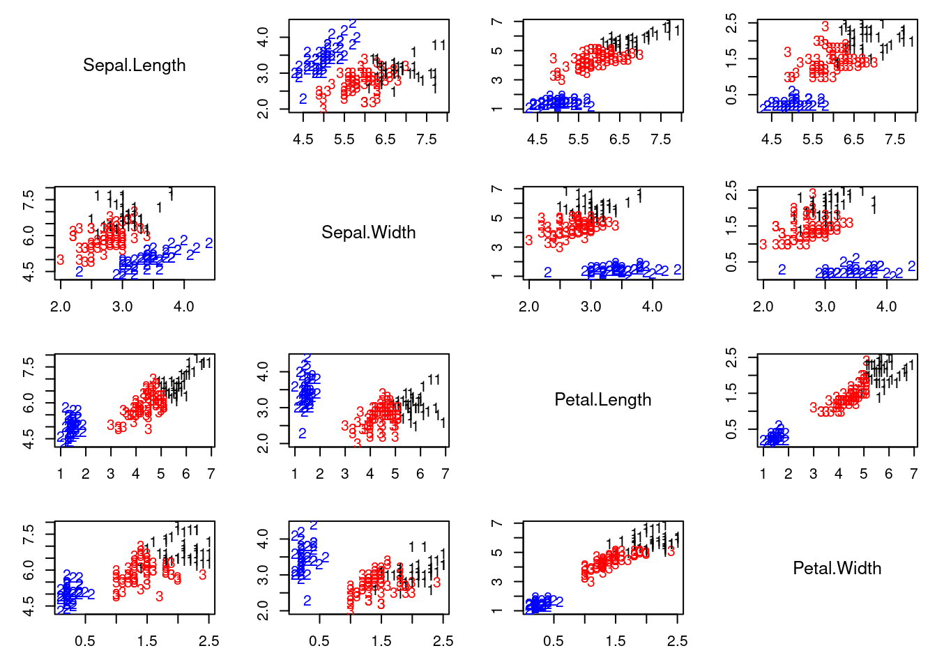
## Cluster reconstruction under the K-means algorithm
irisCluster <- kmeans(x, 3, nstart = numruns)
colscale = c("black","blue","red")
pairs2(x, col=colscale[irisCluster$cluster], labels=irisCluster$cluster)
ARIkmeans = adjustedRandIndex(irisCluster$cluster, as.numeric(iris[,5]))

Figure 74.5: Clustering the iris dataset using k-means clustering and a location and scale mixture model with K normals.

Figure 74.6: Clustering the iris dataset using k-means clustering and a location and scale mixture model with K normals.

Figure 74.7: Clustering the iris dataset using k-means clustering and a location and scale mixture model with K normals.