---
date: 2025-07-07
title: "Bayesian location mixture of AR($p$) models - M3L3"
subtitle: "Bayesian Statistics - Capstone Project"
description: "Capstone Project: Bayesian Conjugate Analysis for Autogressive Time Series Models"
categories:
- Bayesian Statistics
- Capstone Project
keywords:
- Time Series
execute:
freeze: true # never re-render during project render
---
::: {.callout-note collapse="true"}
## Learning Objectives
- [x] Write down the location mixture of AR models under Bayesian conjugate setting. Specify the likelihood function and prior distribution.
- [x] Derive the full conditional distributions and develop the Gibbs sampler for posterior inference of model parameters.
- [x] Implement in the R environment Markov chain Monte Carlo algorithms for fitting mixture models.
:::
## The Location Mixture of AR Models :movie_camera: {#sec-capstone-prediction-location}
Unfortunately the course was missing the video with the derivation of the posterior from the hierarchical model of the location mixture of AR($p$) models. However I have endeavored to fill this in using based on the final reading covering the more sophisticated location and scale mixture of AR($p$).
The location mixture of AR($p$) model for the data can be written hierarchically as follows:
$$
\begin{aligned}
&y_t\sim\sum_{k=1}^K\omega_kN(\mathbf{f}^T_t\boldsymbol{\beta}_k,\nu),\quad \mathbf{f}^T_t=(y_{t-1},\cdots,y_{t-p})^T,\quad t=p+1,\cdots,T\\
&\omega_k\sim Dir(a_1,\cdots,a_k),\quad \boldsymbol{\beta}_k\sim \mathcal{N}(\mathbf{m}_0,\nu_k\mathbf{C}_0),\quad \nu \sim \mathcal{IG}(\frac{n_0}{2},\frac{d_0}{2})
\end{aligned}
$$ {#eq-capstone-loc-arp-mixture}
- where:
- $\mathbf{f}_t$ is the design matrix of the AR model,
- $\boldsymbol{\beta}_k$ is the coefficient vector for the $k$-th component,
- $\nu_k$ is the variance for the $k$-th component, and
- $\omega_k$ is the weight for the $k$-th component.
Introducing a latent configuration variable
$$
\begin{aligned}
L_t &: t \in \{1,2,\cdots,K\} \\
L_t &=k \iff y_t\sim N(\mathbf{f}^T_t\boldsymbol{\beta}_k,\nu)
\end{aligned}
$$ {#eq-capstone-lm-Lt}
We denote: $$
\boldsymbol{\beta}=(\beta_1,\cdots,\beta_K) \qquad \boldsymbol{\omega}=(\omega_1,\cdots,\omega_K)
$$
$$
\mathbf{L}=(L_1,\cdots,L_T)
$$
we can write the full posterior distribution as:
$$
p(\boldsymbol{\beta},\boldsymbol{\nu},\boldsymbol{\omega},\mathbf{L}\mid\mathbf{Y},\mathbf{F}) \propto p(\mathbf{Y}\mid\boldsymbol{\beta},\boldsymbol{\nu},\boldsymbol{\omega},\mathbf{F})p(\boldsymbol{\beta})p(\boldsymbol{\nu})p(\boldsymbol{\omega})p(\mathbf{L})
$$ {#eq-capstone-lm-posterior}
where:
we can write the full posterior distribution as $$
\begin{aligned}
& \mathbb{P}r(\boldsymbol{\omega},\boldsymbol{\beta},\nu,\mathbf{L}|\mathbf{y},\mathbf{F}) \\
&\qquad \propto \mathbb{P}r(\mathbf{y}|\boldsymbol{\omega},\boldsymbol{\beta},\nu,\mathbf{L}) \\
&\qquad\qquad \mathbb{P}r(\mathbf{L}|\boldsymbol{\omega}) \\
&\qquad\qquad \mathbb{P}r(\boldsymbol{\omega}) \\
&\qquad\qquad \mathbb{P}r(\boldsymbol{\beta}) \\
&\qquad\qquad \mathbb{P}r(\nu)\\
&\qquad \propto \prod_{k=1}^K\prod_{\{t:L_t=k\}}N(y_t \mid \mathbf{f}^\top_t\boldsymbol{\beta}_k,\nu)\\
&\qquad \qquad \prod_{k=1}^K\omega_k^{\sum_{t=1}^T\mathbb{I}{(L_t=k)}} \quad \prod_{k=1}^K\omega_k^{a_k-1} \\
&\qquad\qquad\prod_{k=1}^K\left(\mathcal{N}(\boldsymbol{\beta}_k \mid \mathbf{m}_0,\mathbf{C}_0) \ \mathcal{IG}(\nu\mid\frac{n_0}{2},\frac{d_0}{2})\right)
\end{aligned}
$$ {#eq-capstone-lm-posterior-derivation}
$$
\begin{aligned}
\mathbb{P}r(\omega,\beta,L,\nu \mid y) &\propto \prod_{k=1}^K
\underbrace{
\prod_{t:L_t=k} \mathcal{N}(y_t \mid f_t^\top \beta_k,\nu)
}_{
\text{Likelihood of the data } \mid \theta
}\\
&\quad \qquad \underbrace{
\prod_{k=1}^K \omega_k^{\sum_{t=1}^T \mathbb{I}_{(L_t=k)}}
\prod_{k=1}^K \omega_k^{a_k-1}
}_{
\text{Prior for the weights }\omega
}\\
&\quad \qquad \underbrace{
\prod_{k=1}^K \mathcal{N}(\beta_k \mid m_0, \nu C_0)
}_{
\text{Prior for the AR coefficients}
}\\
&\quad \qquad \underbrace{
\mathcal{IG}(\nu \mid \frac{n_0}{2},\frac{d_0}{2})
}_{
\text{Prior for the variance }\nu
}
\end{aligned}
$$ {#eq-capstone-lm-posterior-annotated}
{#fig-capstone-lm-formulas .column-margin group="slides" width="53mm"}
## Full conditional distributions of model parameters :movie_camera: {#sec-capstone-fc}
{#fig-capstone-lm-posterior .column-margin group="slides" width="53mm"}
$$
\begin{aligned}
\mathbb{P}r(\omega,\beta,L,\nu \mid y) &\propto \prod_{k=1}^K
\underbrace{
\prod_{t:L_t=k} \mathcal{N}(y_t \mid f_t^\top \beta_k,\nu)
}_{
\text{Likelihood of the data } \mid \theta
}\\
&\quad \qquad \underbrace{
\prod_{k=1}^K \omega_k^{\sum_{t=1}^T \mathbb{1}_{(L_t=k)}}
\prod_{k=1}^K \omega_k^{a_k-1}
}_{
\text{Prior for the weights }\omega
}\\
&\quad \qquad \underbrace{
\prod_{k=1}^K \mathcal{N}(\beta_k \mid m_0, \nu C_0)
}_{
\text{Prior for the AR coefficients}
}\\
&\quad \qquad \underbrace{
\mathcal{IG}(\nu \mid \frac{n_0}{2},\frac{d_0}{2})
}_{
\text{Prior for the variance }\nu
}
\end{aligned}
$$ {#eq-capstone-lm-full-conditional}
{#fig-capstone-lm-weights .column-margin group="slides" width="53mm"}
$$
\begin{aligned}
\mathbb{P}r(\omega,\beta,L,\nu \mid y) &\propto \prod_{k=1}^K
\underbrace{
\prod_{t:L_t=k} \mathcal{N}(y_t \mid f_t^\top \beta_k,\nu)
}_{
\text{Likelihood of the data } \mid \theta
}\\
&\quad \qquad \underbrace{
\color{blue}\prod_{k=1}^K \omega_k^{\sum_{t=1}^T \mathbb{1}_{(L_t=k)}}
\color{blue}\prod_{k=1}^K \omega_k^{a_k-1}
}_{
\text{Prior for the weights }\omega
}\\
&\quad \qquad \underbrace{
\prod_{k=1}^K \mathcal{N}(\beta_k \mid m_0, \nu C_0)
}_{
\text{Prior for the AR coefficients}
}\\
&\quad \qquad
\underbrace{
\mathcal{IG}(\nu \mid \frac{n_0}{2},\frac{d_0}{2})
}_{
\text{Prior for the variance }\nu
}
\end{aligned}
$$
$$
\begin{aligned}
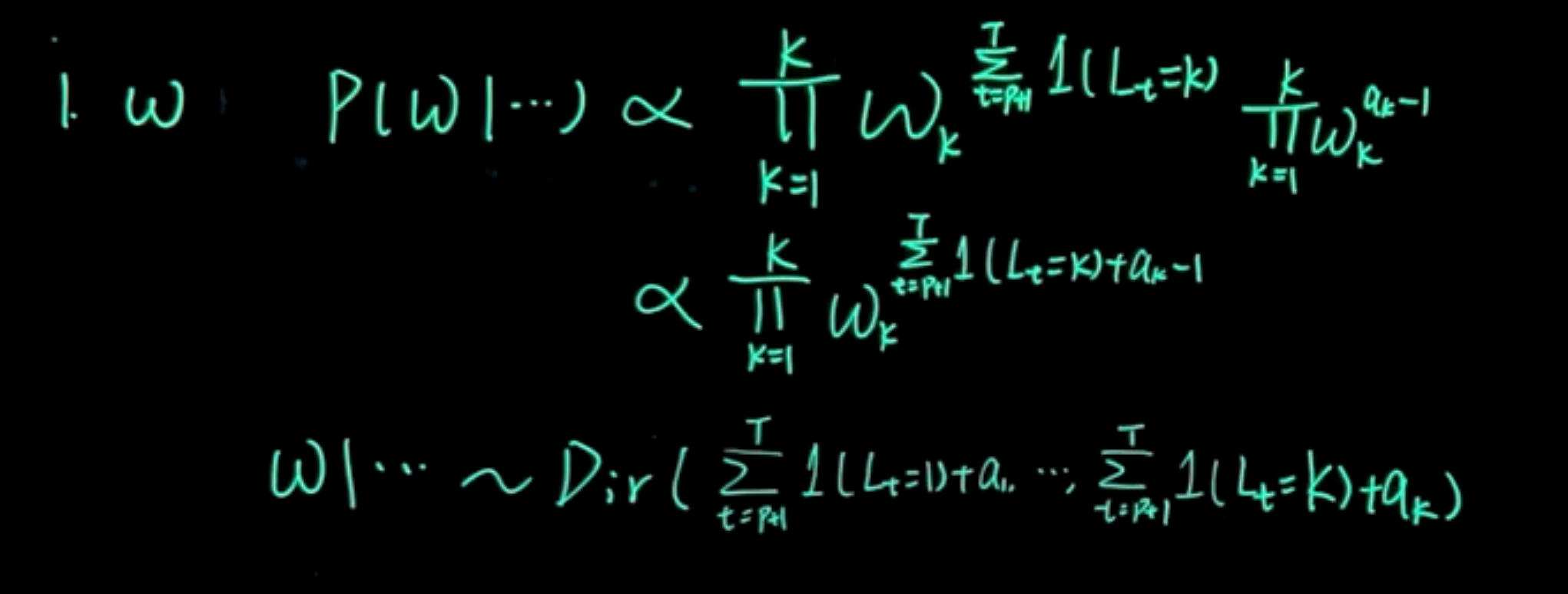
\omega: \quad \mathbb{P}r(\omega\mid\cdots) &\sim
\prod_{k=1}^K \omega_k^{\sum_{t=1}^T \mathbb{1}_{(L_t=k)}}
\prod_{k=1}^K \omega_k^{a_k-1} \\
&\sim \prod_{k=1}^K \omega_k^{\sum_{t=1}^T \mathbb{1}_{(L_t=k)}+a_k-1} \\
&\sim Dir(a_1+\sum_{t=1}^T \mathbb{1}_{(L_t=1)}, \ldots, a_K+\sum_{t=1}^T \mathbb{1}_{(L_t=K)})
\end{aligned}
$$ {#eq-capstone-lm-omega-full-conditional}
{#fig-capstone-lm-ar .column-margin group="slides" width="53mm"}
$$
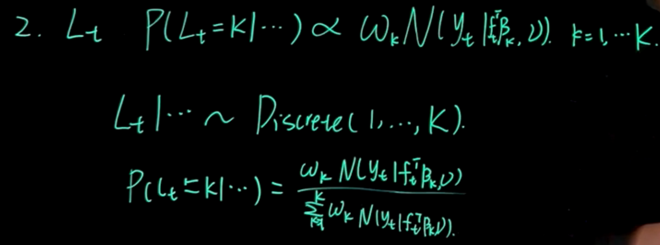
L_t: \quad \mathbb{P}r(L_t=k \mid \cdots) \sim \omega_k \mathcal{N}(y_t \mid f_t^\top \beta_k, \nu) \quad k=1,\ldots,K
$$ {#eq-capstone-lm-Lt-full-conditional}
$$
L_t| \cdots \sim \textrm{Discrete}(1,\ldots,K)
$$ {#eq-capstone-lm-Lt-discrete}
$$
Pr(L_t=k \mid \cdots) = \frac{\omega_k \mathcal{N}(y_t \mid f_t^\top \beta_k, \nu)}{\sum_{j=1}^K \omega_j \mathcal{N}(y_t \mid f_t^\top \beta_j, \nu)}
$$ {#eq-capstone-lm-Lt-probability}
{#fig-capstone-lm-nu .column-margin group="slides" width="53mm"}
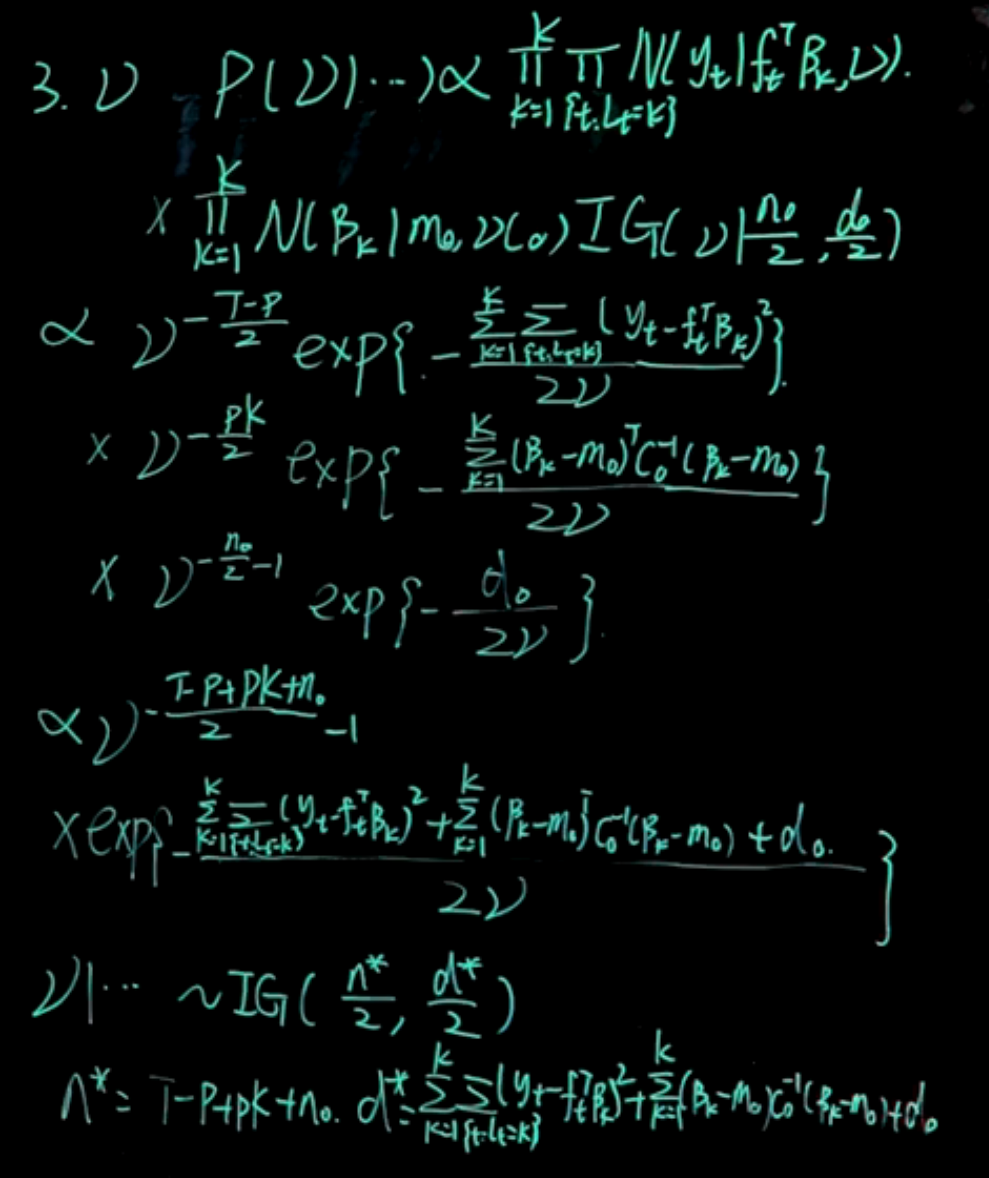
$$
\begin{aligned}
\mathbb{P}r(\nu \mid \cdots) &\propto
\prod_{k=1}^K
\prod_{t:L_t=k} \mathcal{N}(y_t \mid f_t^\top \beta_k,\nu) \\
& \qquad \prod_{k=1}^K \mathcal{N}(\beta_k \mid m_0, \nu C_0)\quad \mathcal{IG}(\nu \mid \frac{n_0}{2},\frac{d_0}{2}) \\
& \propto \nu^{-\frac{T-p}{2}} \exp\left( -\frac{\sum_{k=1}^K \sum_{t:L_t=k} (y_t - f_t^\top \beta_k)^2}{2\nu}\right) \\
& \quad \nu ^ {-\frac{pK}{2}} \exp\left( -\frac{1}{2\nu}\sum_{k=1}^K (\beta_k - m_0)^\top C_0^{-1} (\beta_k-m_0) (\beta_k - m_0)\right) \\
& \quad \nu ^{-\frac{n_0}{2} -1} \exp\left( -\frac{d_0}{2\nu}\right)\\
& \propto \nu^{-\frac{T-p+pK+n_0}{2}-1}
\exp\left( -\frac{ \sum_{k=1}^K\sum_{t:L_t=k} (y_t - f_t^\top \beta_k)^2
+\sum_{k=1}^K (\beta_k - m_0)^\top C_0^{-1} (\beta_k - m_0) +d_0 }{2\nu}\right)
\end{aligned}
$$
$$
\nu \mid \cdots \sim \mathcal{IG}\left(\frac{n^*}{2}, \frac{d^*}{2}\right)
$$
$$
n^* = T - p + n_0 \quad d^* = d_0 + \sum_{k=1}^K \sum_{t:L_t=k} (y_t - f_t^\top \beta_k)^2
$$
{#fig-capstone-lm-beta .column-margin group="slides" width="53mm"}
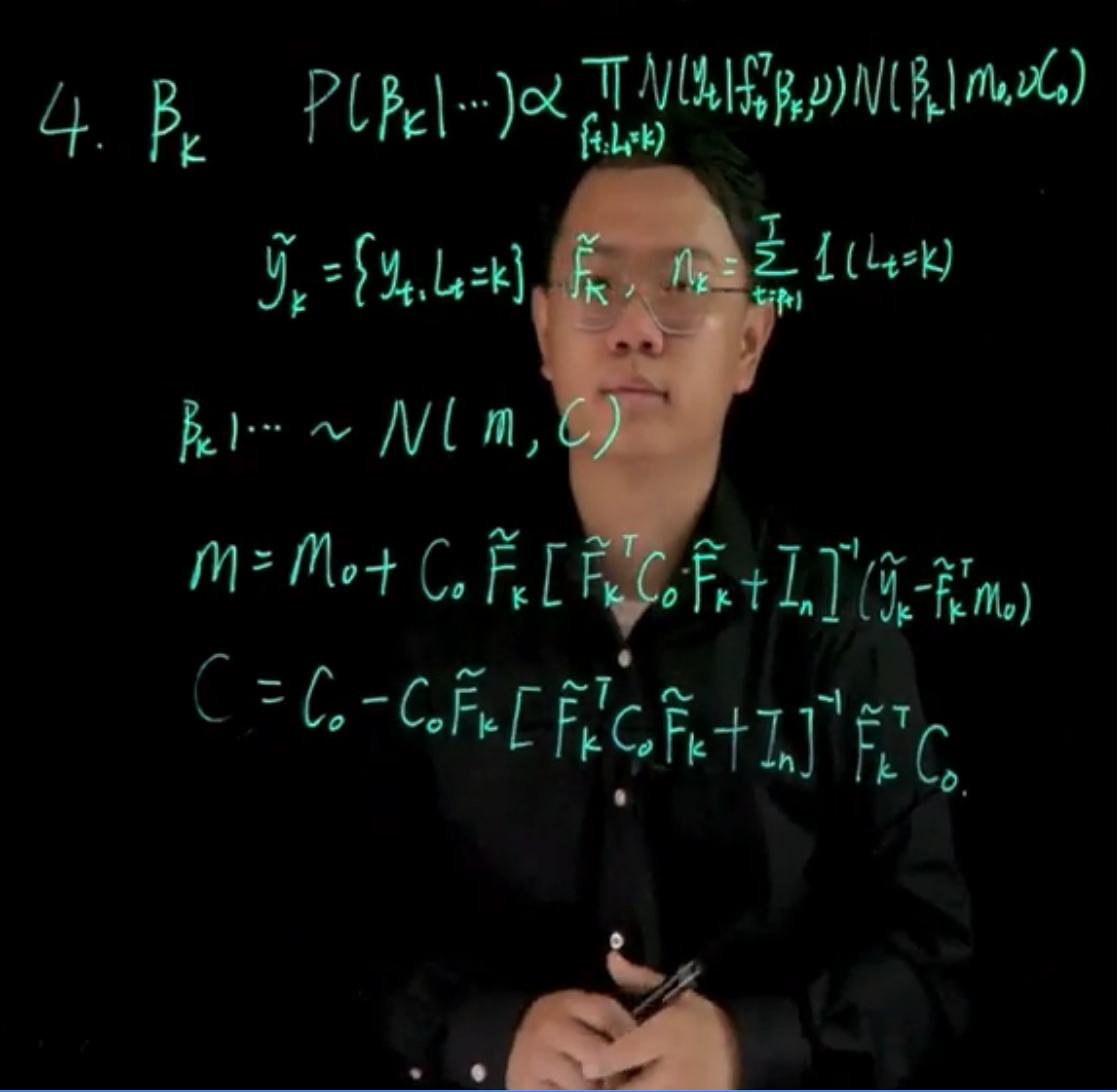
$$
\begin{aligned}
\mathbb{P}r(\beta_k \mid \cdots) &\propto
\prod_{t:L_t=k} \mathcal{N}(y_t \mid f_t^\top \beta_k,\nu)
\mathcal{N}(\beta_k \mid m_0, \nu C_0) \\
\end{aligned}
$$
We can think of this as a single component AR($p$) model using only the part of data that satisfies this $L_t=k$ criteria. $$
\tilde{y}_k = y_{t:L_t=k} \qquad \tilde{F}_k \qquad n_k = \sum_{t:L_t=k} \mathbb{1}_{(L_t=k)}
$$
$$
\beta_k \mid \cdots \sim \mathcal{N}(m_k, C_k)
$$
$$
m = m_0 + C_0 \tilde{F}_k [\tilde{F}_k^\top C_0 \tilde{F}_k + I_n]^{-1} (\tilde{y}_k - \tilde{F}_k^\top m_0)
$$
$$
C = C_0 - C_0 \tilde{F}_k^\top [\tilde{F}_k C_0 \tilde{F}_k^\top + I_n]^{-1} \tilde{F}_k C_0
$$
{#fig-capstone-lm-summary .column-margin group="slides" width="53mm"}
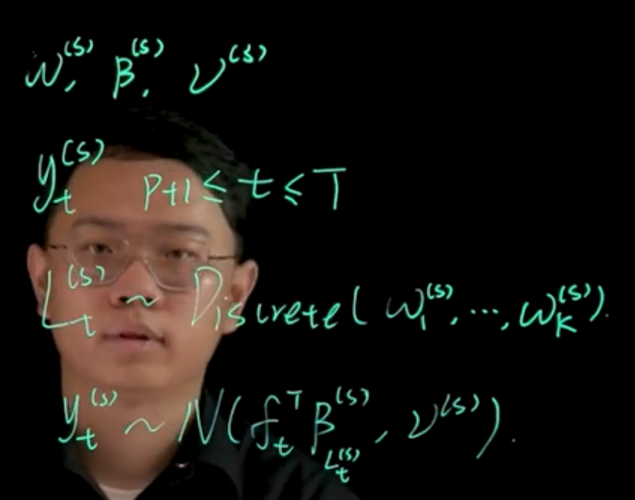
After we obtain posterior samples of model parameters, it is obvious to get ensemble posterior predictions.
$$
\begin{aligned}
\omega^{(s)} \quad \beta^{(s)} \quad \nu^{(s)} \\
y_t^{(s)} \quad p+1 \leq t \leq T \\
L_t^{(s)} \sim Discrete(\omega^{(s)})\\
y_t^{(s)} \sim N(f_t^\top \beta_{L_t^{(s)}},\nu_{L_t^{(s)}})
\end{aligned}
$$
{.column-margin group="slides" width="53mm"}
In this class, we will discuss the Gibbs sampler for obtaining posterior samples of model parameters as well as obtaining in-sample posterior predictions. Last time, we have derived for the mixture model, the full posterior distribution of model parameters have these huge form. We will start from here to find the full conditional distributions for each parameter. Let us start with the weight vector $\omega$. The full posterior distribution of $\omega^{(s)} \mid \cdots$, we will use this three dot to represent the correct conditioning.
Remember, to calculate full conditional distributions, we will select out from this full posterior distribution the specific terms that contains the variable of interest. Trying to recognize those terms as forming a kernel of a family that we know and can recognize.
This is a form of the kernel of the Dirichlet distribution.
## Coding the Gibbs sampler
In this section we walk through some of the code in the next section.
## Sample code for the Gibbs sampler {#sec-capstone-lm-gibbs}
### Step 1 Simulate data
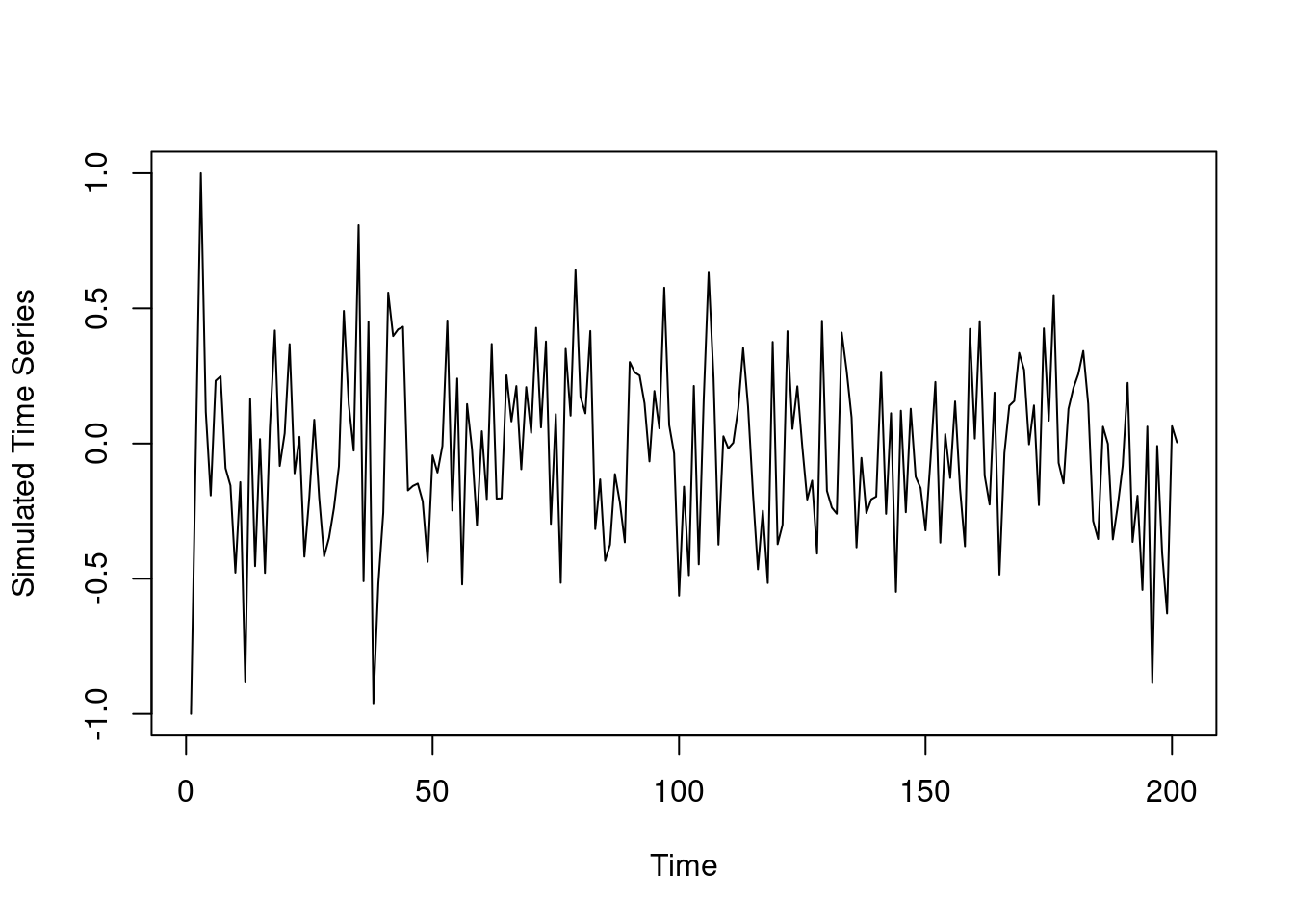
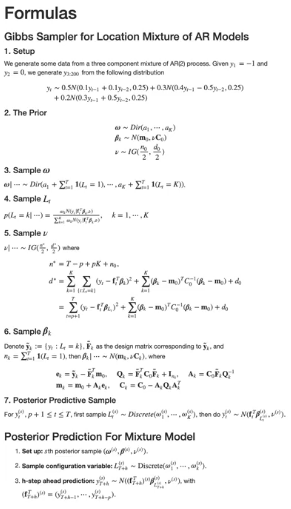
We generate some data from the three component mixture of AR(2) process Given $y_1=-1$ and $y_2=0$ we generate $y_3$ to $y_{3:200}$ from the following distribution:
$$
\begin{aligned}
y_i \sim 0.5\ \mathcal{N}(0.1 y_{t-1} + 0.1 y_{t-2}, 0.25) \\
+\ 0.3\ \mathcal{N}(0.4 y_{t-1} - 0.5 y_{t-2}, 0.25) \\
+\ 0.2\ \mathcal{N}(0.3 y_{t-1} + 0.5 y_{t-2}, 0.25)
\end{aligned}
$$
```{r}
#| label: lst-capstone-lm-sim
## simulate data
y=c(-1,0,1)
n.all =200

for (i in 3:n.all) {
  set.seed(i)
  U=runif(1)
  if(U<=0.5){
    y.new=rnorm(1,0.1*y[i-1]+0.1*y[i-2],0.25)
  }else if(U>0.8){
    y.new=rnorm(1,0.3*y[i-1]+0.5*y[i-2],0.25)
  }else{
    y.new=rnorm(1,0.4*y[i-1]-0.5*y[i-2],0.25)
  }
  y=c(y,y.new)
}


plot(y,type='l',xlab='Time',ylab='Simulated Time Series')
```
### The prior
$$
\begin{aligned}
\omega &\sim Dir(a_1 \ldots a_k) \\
\beta_i &\sim \mathcal{N}(\mathbf{m}_0,\nu \mathbf{C}_0) \\
\nu &\sim \mathcal{IG}(n_0/2,d_0/2)
\end{aligned}
$$ {#eq-capstone-lm-prior}
```{r}
#| label: lst-capstone-lm-gibbs-setup
## Model setup

library(MCMCpack) ## for dirichlet distribution
library(mvtnorm)  ## for multivariate normal distribution


p=2 ## order of AR process
K=3 ## number of mixing component
Y=matrix(y[3:200],ncol=1) ## y_{p+1:T}
Fmtx=matrix(c(y[2:199],y[1:198]),nrow=2,byrow=TRUE) ## design matrix F
n=length(Y) ## T-p

## prior hyperparameters
m0=matrix(rep(0,p),ncol=1) # weakly informative prior
C0=10*diag(p)
C0.inv=0.1*diag(p)
n0=0.02
d0=0.02
a=rep(1,K) ##  parameter for dirichlet distribution
```
```{r}
#| label: lst-capstone-lm-initilize-gibbs
#### MCMC setup
## number of iterations
nsim=20000 # <1>
## store parameters
beta.mtx =matrix(0,nrow=p*K,ncol=nsim) # <2>
L.mtx =matrix(0,nrow=n,ncol=nsim) # <3>
omega.mtx=matrix(0,nrow=K,ncol=nsim) # <4>
nu.vec =rep(0,nsim)
## initial value
beta.cur=rep(0,p*K) # <5>
L.cur=rep(1,n) # <6>
omega.cur=rep(1/K,K) # <7>
nu.cur=1 # <8>
```
1. we want 20,000 samples
2. Each iteration requires $p$ coefficients for $K$ components, and there is one column per iteration.
3. `L.mtx` will be a vector of length n, and there is one column per iteration.
4. The weights omega will be a vector of length K, and there is one column per iteration.
5. We init $\beta$ as 0 which means we assume all coefficients are 0 at the beginning.
6. We init `L.cur` as 1, assigning all observations initially to the first component.
7. We init the weights equally as 1/K, the number components,
8. We init the variance $\nu$ as 1
### Helper functions to sample the full conditional distributions:
We use the following equations to sample from the full conditional
#### To sample for the weights $\omega$
The full conditional for $\omega$ is given by:
$$
\begin{aligned}
\omega \mid \cdots &\sim Dir(a_1+\sum_{t=1}^T \mathbb{1}_{(L_t=1)}, \ldots, a_K+\sum_{t=1}^T \mathbb{1}_{(L_t=K)})
\end{aligned}
$$ {#eq-capstone-lm-omega-full-conditional}
which we implement as follows:
```{r}
#| label: lst-capstone-lm-gibbs-helpers-omega
#### sample functions
sample_omega=function(L.cur){ # <1>
n.vec=sapply(1:K, function(k){sum(L.cur==k)})
rdirichlet(1,a+n.vec)
} # <1>
```
1. this samples $\omega$ using a Dirichlet RV parametrized by vector of sum of indicators from the current latent vars `L.cur`
note that the `sample_omega` takes a parameter `L.cur` which is the current latent variable vector.
This is used to count how many observations are assigned to each component.
#### To sample the latent variable $L_t$
$$
Pr(L_t=k \mid \cdots) = \frac{\omega_k \mathcal{N}(y_t \mid f_t^\top \beta_k, \nu)}{\sum_{j=1}^K \omega_j \mathcal{N}(y_t \mid f_t^\top \beta_j, \nu)} \qquad k \in 1:K
$$
```{r}
#| label: lst-capstone-lm-gibbs-helpers-L
sample_L_one=function(beta.cur,omega.cur,nu.cur,y.cur,Fmtx.cur){ # <2>
prob_k=function(k){
beta.use=beta.cur[((k-1)*p+1):(k*p)]
omega.cur[k]*dnorm(y.cur,mean=sum(beta.use*Fmtx.cur),sd=sqrt(nu.cur))
}
prob.vec=sapply(1:K, prob_k)
L.sample=sample(1:K,1,prob=prob.vec/sum(prob.vec))
return(L.sample)
} # <2>
sample_L=function(y,x,beta.cur,omega.cur,nu.cur){ #<3>
L.new=sapply(1:n, function(j){sample_L_one(beta.cur,omega.cur,nu.cur,y.cur=y[j,],Fmtx.cur=x[,j])})
return(L.new)
} # <3>
```
2. to sample the Configuration variable $L$ probability of each **one** $L_k$ for a single observation $y_t$
3. this samples the latent variable for all observations
#### To sample $\nu$
$$
\begin{aligned}
\mathbb{P}r(\nu \mid \cdots) & \sim \mathcal{IG}(\nu \mid \frac{n^*}{2},\frac{d^*}{2}) \\
n^* &= T - p + n_0 \\
d^* &= \sum_{t:L_t=k} (y_t - f_t^\top \beta_k)^2 + \sum_{k=1}^K (\beta_k-m_0)^\top C_0^{-1} (\beta_k-m_0) + d_0
\end{aligned}
$$
```{r}
#| label: lst-capstone-lm-gibbs-helpers-nu
sample_nu=function(L.cur,beta.cur){ # <4>
err.y=function(idx){
L.use = L.cur[idx]
beta.use = beta.cur[((L.use-1)*p+1):(L.use*p)]
err = Y[idx,]-sum(Fmtx[,idx]*beta.use)
return(err^2)
}
n.star=n0+n
d.star = d0+sum(sapply(1:n,err.y))
1/rgamma(1,shape=n.star/2,rate=d.star/2)
} # <4>
```
4. this samples the variance parameter
```{r}
#| label: lst-capstone-lm-gibbs-helpers-beta
sample_beta=function(k,L.cur,nu.cur){ # <5>
idx.select=(L.cur==k)
n.k=sum(idx.select)
if(n.k==0){
m.k=m0
C.k=C0
}else{
y.tilde.k=Y[idx.select,]
Fmtx.tilde.k=Fmtx[,idx.select]
e.k=y.tilde.k-t(Fmtx.tilde.k)%*%m0
Q.k=t(Fmtx.tilde.k)%*%C0%*%Fmtx.tilde.k+diag(n.k)
Q.k.inv=chol2inv(chol(Q.k))
A.k=C0%*%Fmtx.tilde.k%*%Q.k.inv
m.k=m0+A.k%*%e.k
C.k=C0-A.k%*%Q.k%*%t(A.k)
}
rmvnorm(1,m.k,nu.cur*C.k)
} # <5>
```
5. this samples the weights
#### To sample $\beta$:
- We denote :
- $\tilde{y}_k := \{y_t : L_t=k\}$
- $\tilde{F}_k$ as the design matrix corresponding to $\tilde{y}_k$
- $n_k = \sum_{t=1}^K \mathbb{I}_{(L_t=k)}$
$$
\beta_k \mid \cdots \sim \mathcal{N}(\mathbf{m}_k, \nu \mathbf{C}_k)
$$
where:
$$
\begin{aligned}
\mathbf{m}_k &= \mathbf{m}_0+\mathbf{A}_k\mathbf{e}_k,
&\mathbf{C}_k &= \mathbf{C}_0-\mathbf{A}_k\mathbf{Q}_k\mathbf{A}_k^{T} \\
\mathbf{e}_k &= \mathbf{\tilde{y}}_k-\mathbf{\tilde{F}}_k^T\mathbf{m}_0,
&\mathbf{Q}_k &= \mathbf{\tilde{F}}_k^T\mathbf{C}_0\mathbf{\tilde{F}}_k+\mathbf{I}_{n_k}, \\
\mathbf{A}_k &= \mathbf{C}_0\mathbf{\tilde{F}}_k\mathbf{Q}_k^{-1} \\
n_k^* &= n_0+n_k,
&d_k^* &= d_0+\mathbf{e}_k^T\mathbf{Q}_k^{-1}\mathbf{e}_k
\end{aligned}
$$
```{r}
#| label: lst-capstone-lm-gibbs-sampler-beta
## Gibbs Sampler

for (i in 1:nsim) {
  set.seed(i)

  ## sample omega
  omega.cur=sample_omega(L.cur)
  omega.mtx[,i]=omega.cur

  ## sample L
  L.cur=sample_L(Y,Fmtx,beta.cur,omega.cur,nu.cur)
  L.mtx[,i]=L.cur

  ## sample nu
  nu.cur=sample_nu(L.cur,beta.cur)
  nu.vec[i]=nu.cur

  ## sample beta
  beta.cur=as.vector(sapply(1:K, function(k){sample_beta(k,L.cur,nu.cur)}))
  beta.mtx[,i]=beta.cur

  ## show the numer of iterations
  if(i%%1000==0){
    print(paste("Number of iterations:",i))
  }

}
#### show the result
sample.select.idx=seq(10001,20000,by=1)
post.pred.y.mix=function(idx){
k.vec.use=L.mtx[,idx]
beta.use=beta.mtx[,idx]
nu.use=nu.vec[idx]
get.mean=function(s){
k.use=k.vec.use[s]
sum(Fmtx[,s]*beta.use[((k.use-1)*p+1):(k.use*p)])
}
mu.y=sapply(1:n, get.mean)
sapply(1:length(mu.y), function(k){rnorm(1,mu.y[k],sqrt(nu.use))})
}
y.post.pred.sample=sapply(sample.select.idx, post.pred.y.mix)
summary.vec95=function(vec){
c(unname(quantile(vec,0.025)),mean(vec),unname(quantile(vec,0.975)))
}
summary.y=apply(y.post.pred.sample,MARGIN=1,summary.vec95)
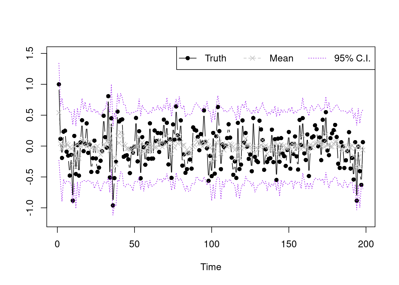
plot(Y,type='b',xlab='Time',ylab='',pch=16,ylim=c(-1.2,1.5))
lines(summary.y[2,],type='b',col='grey',lty=2,pch=4)
lines(summary.y[1,],type='l',col='purple',lty=3)
lines(summary.y[3,],type='l',col='purple',lty=3)
legend("topright",legend=c('Truth','Mean','95% C.I.'),lty=1:3,
col=c('black','grey','purple'),horiz = T,pch=c(16,4,NA))
```