It is often pointed out that Normally distributed data is not very commonly encountered in the real world. However, when it comes to modeling, using a normal RV is second to none.(Hoff 2009, 75). The Section F.1 is the primary reason that the normal is a good approximation if there are enough IID samples. We will look at two types of conjugate normal priors, and in the next unit we will consider two more uninformative priors for Normally distributed data.
Charles Zaiontz provides pro types of conjugate priors for normally distributed data:
- Mean unknown and variance known.
- Variance unknown and mean known and
- Mean and variance are unknown
In each case, the unknown refer to population statistics. Since we are able to estimate sample parameters such as the mean and variance quite easily. A key question to consider is how well does our posterior distribution of the parameter representative of the unknown population statistic?
Ideally, I will update the notes below with proofs of conjugate, prior and posterior and marginal distribution.
Some of the proofs are in here as well
- See (Gelman et al. 2013, sec. 3.2) for Normal data with a noninformative prior distribution
- See (Gelman et al. 2013, sec. 3.2) for Normal data with a conjugate prior distribution
23.1 Normal Likelihood with known variance
Note: this material is also covered in (Hoff 2009, sec. 5.2)
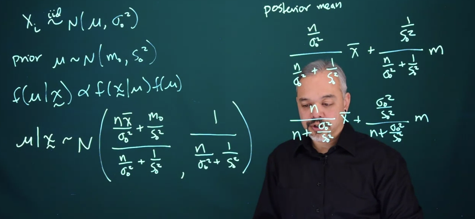
Let’s suppose the standard deviation or variance \sigma^2 is known and we’re only interested in learning about the mean. This is a situation that often arises in monitoring industrial production processes.
X_i \stackrel{iid}\sim \mathcal{N}(\mu, \sigma^2) \tag{23.1}
It turns out that the Normal distribution is conjugate for itself when looking for the mean parameter
Prior
\mu \sim \mathcal{N}(m_0,S_0^2) \tag{23.2}
By Bayes rule:
f(\mu \mid x ) \propto f(x \mid \mu)f(\mu)
\mu \mid x \sim \mathcal{N} \left (\frac{\frac{n\bar{x}}{\sigma_0^2} + \frac{m_0}{s_0^2} }{\frac{n}{\sigma_0^2} +\frac{1}{s_0^2}}, \frac{1}{\frac{n}{\sigma_0^2} + \frac{1}{s_0^2}}\right ) \tag{23.3}
where:
- n is the sample size
- \bar{x}=\frac{1}{n}\sum x_i is the sample mean
- \sigma =\frac{1}{n} \sum (x_i-\bar{x})^2 is the sample variance
- indexing parameters with 0 seems to be a convention that they are from the prior:
- s_0 is the prior variance
- m_0 is the prior mean
Let’s look at the posterior mean
\begin{aligned} posterior_{\mu} &= \frac{ \frac{n}{\sigma_0^2}} {\frac{n}{\sigma_0^2}s + \frac{1}{s_0^2}}\bar{x} + \frac{ \frac{1}{s_0^2} }{ \frac{n}{\sigma_0^2} + \frac{1}{s_0^2} }m \\ &= \frac{n}{n + \frac{\sigma_0^2}{s_0^2} }\bar{x} + \frac{ \frac{\sigma_0^2}{s_0^2} }{n + \frac{\sigma_0^2}{s_0^2}}m \end{aligned} \tag{23.4}
should we use n-1 in the sample variance?
Thus we see, that the posterior mean is a weighted average of the prior mean and the data mean. And indeed that the effective sample size for this prior is the ratio of the variance for the data to the variance in the prior.
Prior\ ESS= \frac{\sigma_0^2}{s_0^2} \tag{23.5}
This makes sense, because the larger the variance of the prior, the less information that’s in it.
The marginal distribution for Y is
\mathcal{N}(m_0, s_0^2 + \sigma^2) \tag{23.6}
23.1.1 Prior (and posterior) predictive distribution
The prior (and posterior) predictive distribution for data is particularly simple in the conjugate normal model .
If y \mid \theta \sim \mathcal{N}(\theta,\sigma^2) and \theta \sim \mathcal{N}(m, s_0^2)
then the marginal distribution for Y, obtained as
\int f(y,\theta) d\theta = \mathcal{N}(m_0,s_0^2) \tag{23.7}
Example 23.1 Suppose your data are normally distributed with \mu=\theta and \sigma^2=1.
y \mid \theta \sim \mathcal{N}(\theta,1)
You select a normal prior for \theta with mean 0 and variance 2.
\theta \sim \mathcal{N}(0, 2)
Then the prior predictive distribution for one data point would be N(0, a). What is the value of a?
Since, m_0 =0, and s^2_0=2 and \sigma^2=1, the predictive distribution is N(0,2+1).
23.2 Normal likelihood with expectation and variance unknown
This section is challenging.
- The updating derivation is skipped,
- the posterior
- updating rule values are introduced without motivations and explanation.
- The model is also the most complicated in the course, the note at the end says this can be extended hierarchically if we want to specify hyper priors for m, w and \beta
- Other text discuss this case using a inverse chi squared distribution
If we can understand the model the homework is going to make sense. Also this is probably the level needed for the other courses in the specialization.
It can help to review some of the books:
- See (Hoff 2009, sec. 5.3) which has some R examples.
- See (Gelman et al. 2013, sec. 5)
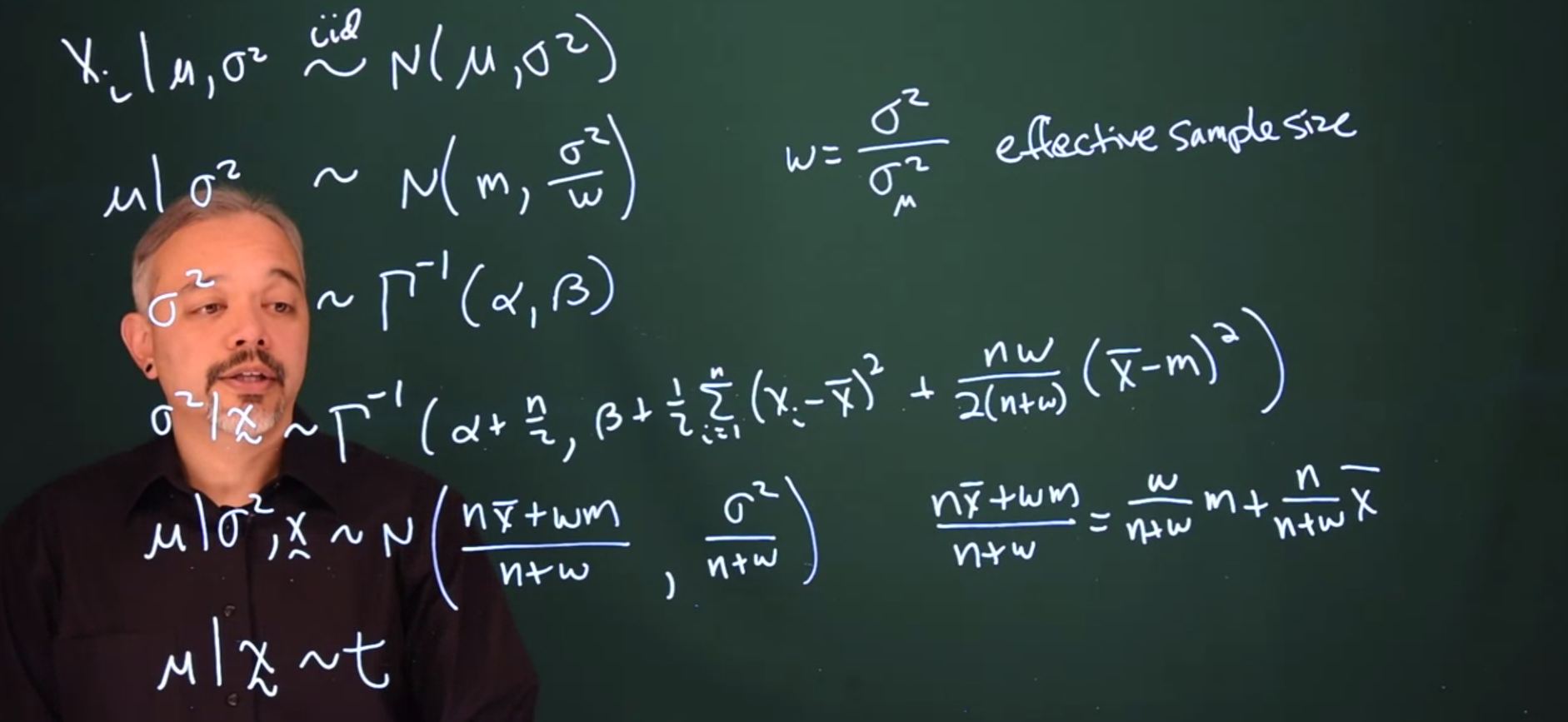
If both \mu and \sigma^2 are unknown, we can specify a conjugate prior in a hierarchical fashion.
X_i \mid \mu, \sigma^2 \stackrel{iid}\sim \mathcal{N}(\mu, \sigma^2) \qquad \text{(the data given the params) }
- This is the level 1 hierarchically model - X_i model our observations.
- We state on the left, that the RV X is conditioned on the \mu and \sigma^2.
- But the variables \mu and \sigma^2 are unknown population statistics which we will need to infer from the data. We can call them latent variables.
Next we add a prior from \mu conditional on the value for \sigma^2
\mu \mid \sigma^2 \sim \mathcal{N}(m, \frac{\sigma^2}{w}) \qquad \text{(prior of the mean conditioned on the variance)}
where:
- w is going to be the ratio of \sigma^2 and some variance for the Normal distribution. This is the effective sample size of the prior.
- Why is the mean conditioned on the variance. We can have a model where they are independent too?
- later on (in the homework) we are told that w can express the confidence in the prior.
- I think this means that Since this is a knowledge of m, i.e. giving w a weight of 1/10 expresses that we value
- Perhaps this is due to Central Limit Theorem ?
- This is level 2 of the model
Finally, the last step is to specify a prior for \sigma^2. The conjugate prior here is an inverse gamma distribution with parameters \alpha and \beta.
\sigma^2 \sim \mathrm{Gamma}^{-1}(\alpha, \beta) \qquad \text{prior of the variance}
After many calculations… we get the posterior distribution
\sigma^2 \mid x \sim \mathrm{Gamma}^{-1}(\alpha + \frac{n}{2}, \beta + \frac{1}{2}\sum_{i = 1}^n{(x-\bar{x}^2 + \frac{nw}{2(n+2)}(\bar{x} - m)^2)}) \tag{23.8}
\mu \mid \sigma^2,x \sim \mathcal{N}(\frac{n\bar{x}+wm}{n+w}, \frac{\sigma^2}{n + w}) \tag{23.9}
Where the posterior mean can be written as the weighted average of the prior mean and the data mean.
\frac{n\bar{x}+wm}{n+w} = \frac{w}{n + w}m + \frac{n}{n + w}\bar{x} \qquad \text{post. mean} \tag{23.10}
In some cases, we only care about \mu. We want some inference on \mu and we may want it such that it does not depend on \sigma^2. We can marginalize that \sigma^2 integrating it out. The posterior for \mu marginally follows a t distribution.
\mu \mid x \sim t
Similarly, the posterior predictive distribution also is a t distribution.
Finally, note that we can extend this in various directions, this can be extended to the multivariate normal case that requires matrix vector notations and can be extended hierarchically if we want to specify priors for m, w, \beta