14 Priors - M3L6

In this section, we will delve more deeply into choices of Priors and how they influence Bayesian CI by developing the prior predictive (Definition 14.1) and posterior predictive (Definition 14.2) intervals.

14.1 Priors and prior predictive distributions

ImportantChoosing a prior

How should we choose a prior?

1. Our prior needs to represent our perspectives, beliefs, and our uncertainties.
2. It should encode any constraints on the data or parameters.
   • age is positive and less than 120
3. It can regularize the data
4. It could encode expert knowledge we have elicited from domain experts.
5. It should prefer informative priors over uninformative ones.

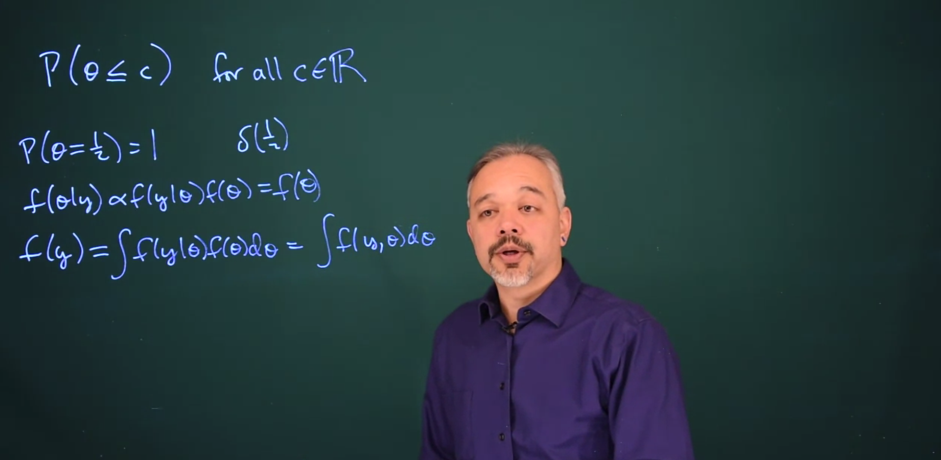
Theoretically, we’re defining a cumulative distribution function for the parameter

\mathbb{P}r(\theta \le c) \qquad \forall c \in \mathbb{R}

We need to do this for an infinite number of possible sets but it isn’t practical to do, and it would be very difficult to do it coherently so that all the probabilities were consistent. Therefore in practice, we tend to work with a convenient family that is flexible enough for members to represent our beliefs.

Generally if one has enough data, the information in the data will overwhelm the information in the prior. This makes it seem like the prior is less important in terms of the form and substance of the posterior. Once the prior is overwhelmed, any reasonable choice of prior will lead to approximately the same posterior. This is a point where the Bayesian approach should converge to the frequentist and can be shown to be more or less objective.

On the other hand choices of priors can be important because even with masses of data, groups and items can be distributed very sparsely in which case priors can have a lasting impact on the posteriors. Secondly, we can decide to pick priors that have a long-lasting impact on operating as regularizing constraints within our models. In such cases, the impact of the prior can be significant.

One of our guiding questions will be to consider how much information the prior and the data contribute to the posterior. We will consider the effective sample size of different priors.

Finally, a bad choice of priors can lead to specific issues.

Example 14.1 (Example of Bad Prior) Suppose we chose a prior that says the probability of \mathbb{P}r(\theta = \frac{1}{2}) = \delta( \frac{1}{2})= 1

And thus, the probability of \theta equaling any other value is 0. If we do this, our data won’t make a difference since we only put a probability of 1 at a single point.

f(\theta \mid y) \propto f(y \mid\theta)f(\theta) = f(\theta) = \delta(\theta) \tag{14.1}

CautionAvoid priors that assign 0 or 1

• Events with a prior probability of 0 will always have a posterior probability of 0 because f(\theta)=0 in (Equation 14.1) the product will and therefore the posterior be 0
• Events with a prior probability of 1, will always have a posterior probability of 1. This is a little harder to see. In this case f(\theta^c)=0 in (Equation 14.1) so that the posterior will again be zero elsewhere.

• It is good practice to avoid assigning a probability of 0 or 1 to any event that has already occurred or is already known not to occur.
• If the priors avoid 0 and 1 values the information within the data will eventually overwhelm the information within the prior.

14.1.1 Calibration - making priors precise

Q. How do we calibrate our prior probability to reality?

Calibration of predictive intervals is a useful concept in terms of choosing priors. If we make an interval where we’re saying we predict 95% of new data points will occur in this interval. It would be good if, in reality, 95% of new data points did fall in that interval. This is a frequentist concept but this is important for practical statistical purposes so that our results reflect reality.

Figure 14.1: Prior Predictive Distribution

We can compute a predictive interval. This is an interval such that 95% of new observations are expected to fall into it. It’s an interval for the data rather than an interval for \theta

Definition 14.1 (Prior Predictive Distribution) The prior predictive distribution expresses our uncertainty about a parameter, i.e. the distribution of its possible values before we observe any data.

\begin{aligned} f(y) &= \int{f(y \mid\theta)f(\theta)d\theta} &&\text {by Bayes theorem} \\&= \int{f(y, \theta)d\theta} && \text{the joint probability} \end{aligned} \tag{14.2}

• f(y,\theta) is the joint density of y and \theta.
• If we are integrating out \theta, we will end up with a marginalized probability distribution of the data.
• However, we may well decide to not integrate out \theta completely, so we will end up with a predictive interval.
• But no data y has been observed, so this is the prior predictive before any data is observed.
• It is used in prior predictive checks to assess whether the choice of prior distribution captures our prior beliefs.

14.2 Prior Predictive: Binomial Example

Figure 14.2: Prior Predictive Distribution Binomial Example

Suppose we’re going to flip a coin 10 times and count the number of heads we see. But we are thinking about this in advance of actually doing it, and we are interested in the predictive distribution

Q. How many heads do we predict we’re going to see?

Q. What’s the probability that it shows up heads?

So, we’ll need to choose a prior.

N=10 \qquad \text {number of coin flips}

Where Y_i represents individual coin flips. with Head being a success

Y \sim \text{Bernoulli}(\theta)

Our data is the count of successes (heads) in N flips.

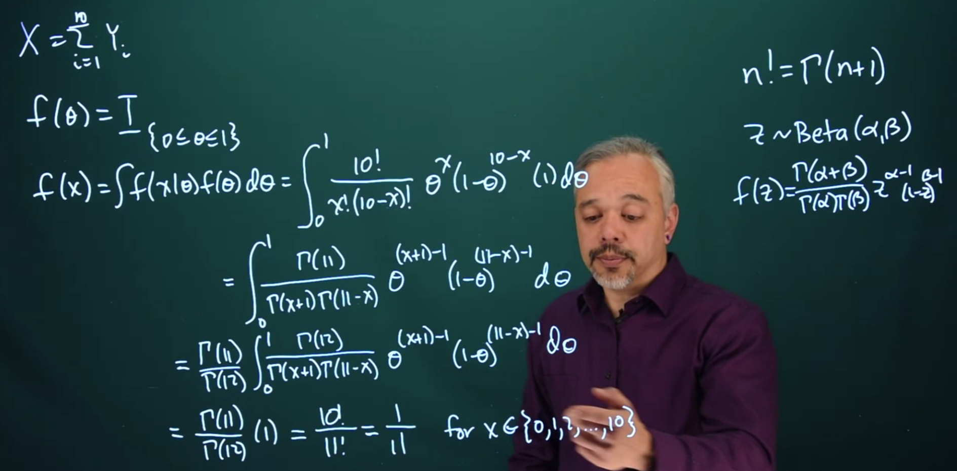
X = \sum_{i=0}^N Y_i \qquad

If we think that all possible coins or all possible probabilities are equally likely, then we can put a prior for \theta that’s flat over the interval from 0 to 1. That is the Uniform prior (Equation 6.17):

f(\theta)=\mathbb{I}_{[0 \le \theta \le 1]}

The predictive probability is a binomial likelihood times the prior = 1

f(x) = \int f(x \mid\theta) f(\theta) d\theta = \int_0^1 \frac{10!}{x!(10-x)!} \theta^x(1-\theta)^{10-x}(1) d \theta

Note that because we’re interested in X at the end, it’s important that we distinguish between a Binomial density and a Bernoulli density. Here we just care about the total count rather than the exact ordering which would be Bernoulli.

For most of the analyses, we’re doing, where we’re interested in \theta rather than x, the binomial and the Bernoulli are interchangeable because the part in here that depends on \theta is the same.

To solve this integral let us recall that:

n! =\Gamma(n+1) \tag{14.3}

and

Z \sim \text{Beta}(\alpha,\beta)

The PDF for the beta distribution is given as:

f(z)= \frac{\Gamma(\alpha+\beta)}{\Gamma(\alpha)\Gamma(\beta)} z^{\alpha−1}(1−z)^{\beta−1}I_{(0 < z <1)}

where \alpha>0 and \beta>0.

\begin{aligned} f(x) &= \int f(x \mid\theta) f(\theta) d\theta && \text {prior predictive dfn} \\ &= \int_0^1 \frac{10!}{x!(10-x)!} \theta^x(1-\theta)^{10-x}( \mathbb{I_{[0,1]}}) d \theta && \text {subst. Binomial, } \mathbb{I_{[0,1]}} \\ &= \int_0^1 \frac{\Gamma(11)}{\Gamma(x+1)\Gamma(11-x)} \theta^{(x+1)-1}(1-\theta)^{(11-x)-1}(1) d \theta && \text {convert to Beta(x+1,11-x), } \\ &=\frac{\Gamma(11)}{\Gamma(12)} \cancel{ \int_0^1 \frac{\Gamma(12)}{\Gamma(x+1)\Gamma(11-x)}\theta^{(x+1)-1}(1-\theta)^{(11-x)-1}(1)d \theta } && \text {integrating PDF=1 } \\ &=\frac{\Gamma(11)}{\Gamma(12)} \times 1 = \frac{10!}{11!} =\frac{1}{11} && \forall x \in \{1,2,\dots,10\} \end{aligned}

Thus we see that if we start with a uniform prior, we then end up with a discrete uniform predictive density for X. If all possible \theta probabilities are equally likely, then all possible sums X outcomes are equally likely.

The integral above is a beta density, all integrals of valid beta densities equal one.

f(x) = \frac{\Gamma(11)}{\Gamma(12)} = \frac{10!}{11!} = \frac{1}{11}

14.3 Posterior Predictive Distribution

Posterior Predictive Distribution

What about after we’ve observed data? What’s our posterior predictive distribution?

Going from the previous example, let us observe after one flip that we got a head.

We want to ask, what’s our predictive distribution for the second flip, given we saw a head on the first flip?

14.4 Posterior Predictive Distribution

The posterior predictive distribution is produced analogously to the posterior predictive distribution by marginalizing the posterior with respect to the parameter.

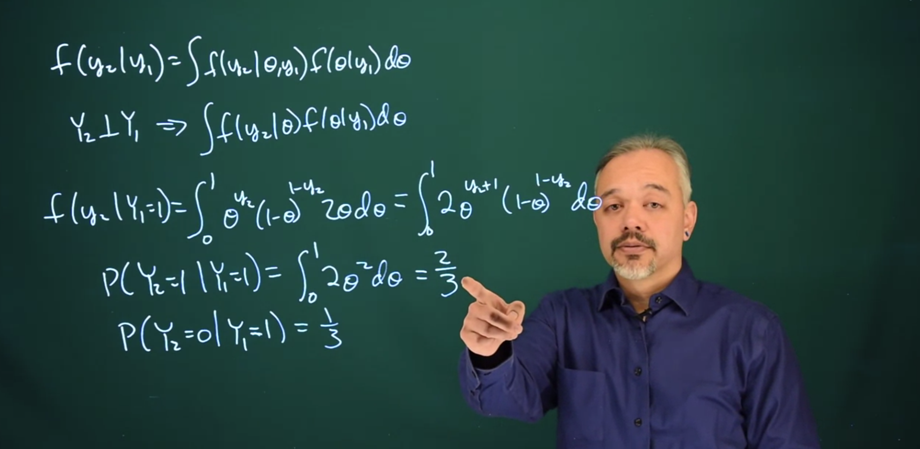
Definition 14.2 (Posterior Predictive Distribution) \begin{aligned} f(y_2 \mid y_1) &= \text{likelihood}\times \text{posterior} \\ &= \int{f(y_2 \mid \theta,y_1) \; f(\theta \mid y_1)}d\theta \end{aligned} \tag{14.4}

TipMarginalizing distribution

Suppose we have an experiment with events based on two RVs: - (C) a coin toss - (D) and a dice toss. And we call this event X = \mathbb{P}r(C,D) = \mathbb{P}r(C) \times \mathbb{P}r(D)

C D	1	2	3	4	5	6	\mathbb{P}r(C)
H	1/12	1/12	1/12	1/12	1/12	1/12	6/12
T	1/12	1/12	1/12	1/12	1/12	1/12	6/12
\mathbb{P}r(D)	2/12	2/12	2/12	2/12	2/12	2/12	1

We can recover the \mathbb{P}r(C) coin’s distribution or the dice distribution \mathbb{P}r(D) by marginalization. \mathbb{P}r(X) This is done by summing over the row or columns.

The marginal distribution let us subset a joint distribution. The marginal distribution has removed the uncertainty due to a parameter.

we use three terms interchangeably :

• marginalizing the posterior w.r.t. \theta
• integrating/summing over \theta
• integrating \theta out

The first is the real idea, the others are the techniques being used to do it. For a predictive distribution we may want to marginalize all the parameters so we end up with the RV we wish to predict.

We’re going to assume that Y_2 is independent of Y_1. Therefore,

f(y_2 \mid y_1) = \int{f(y_2 \mid \theta)f(\theta \mid y_1)d\theta}

Suppose we’re thinking of a uniform distribution for \theta and we observe the first flip is a “head”. What do we predict for the second flip?

This is no longer going to be a uniform distribution like it was before because we have some data. We’re going to think it’s more likely that we’re going to get a second head. We think this because since we observed a head \theta is now likely to be at least \frac{1}{2} possibly larger.

f(y_2 \mid Y_1 = 1) = \int_0^1{\theta^{y_2}(1-\theta)^{1-y_2}2\theta d\theta}

f(y_2 \mid Y_1 = 1) = \int_0^1{2\theta^{y_2 + 1}(1-\theta)^{1-y_2}d\theta}

We could work this out in a more general form, but in this case, Y_2 has to take the value 0 or 1. The next flip is either going to be heads or tails so it’s easier to just plop in a particular example.

\mathbb{P}r(Y_2 = 1 \mid Y_1 = 1) = \int_\theta^1 {2 \theta^2 d \theta} = \frac{2}{3}

\mathbb{P}r(Y_2 = 0 \mid Y_1 = 1) = 1 - \mathbb{P}r(Y_2 = 1 \mid Y_1 = 1) = 1 - \frac{2}{3} = \frac{1}{3}

We can see here that the posterior is a combination of the information in the prior and the information in the data. In this case, our prior is like having two data points, one head and one tail.

Saying we have a uniform prior for \theta is equivalent in an information sense to saying “we have observed one ‘Head’ and one ‘Tail’”.

So then when we observe one head, it’s like we now have seen two heads and one tail. So our predictive distribution for the second flip says if we have two heads and one tail, then we have a \frac{2}{3} probability of getting another head and a \frac{1}{3} probability of getting another tail.