---
date: 2024-11-09
title: "Bayesian Inference in the NDLM: Part 2"
subtitle: Time Series Analysis
description: "Normal Dynamic Linear Models (NDLMs) are a class of models used for time series analysis that allow for flexible modeling of temporal dependencies."
categories:
- Bayesian Statistics
- Time Series
keywords:
- Time series
- Filtering
- Smoothing
- NDLM
- Normal Dynamic Linear Models
- Seasonal NDLM
- Superposition Principle
- R code
fig-caption: Notes about ... Bayesian Statistics
title-block-banner: images/banner_deep.jpg
---
## Filtering, Smoothing and Forecasting: Unknown observational variance :movie_camera: {#section-NDLM-unknown-variance}
::: {.callout-tip collapse="false"}
## Recap:
In [@sec-Bayesian-inference-NDLM-known-variances] we performed Bayesian inference on [@eq-inference-NDLM], an NDLM with known observational variance $\nu_t$ and system variance $\boldsymbol{\omega}_t$ c.f.and determined that under the assumption of a normal prior $(\theta_0 \mid \mathcal{D}_0) \sim \mathcal{N}(\mathbf{m}_{0}, \mathbf{C}_{0})$, with
filtering leads to a posterior $p(\boldsymbol{\theta}_t|\mathcal{D}_t) \sim N (\mathbf{m}_t, \mathbf{C}_t)$
and smoothing leads to normal posterior distributions
In this lesson we will explore the case of the NDLM, where we **assume** That the observational variance $\nu_t=v$ i.e. is constant over time.
:::
### Inference in the NDLM with unknown constant observational variance:
Let $\nu_t = v\ \forall t$ with $\nu$ unknown and consider a DLM with the following structure:
$$
\begin{aligned}
y_t &= \mathbf{F}_t^\top \boldsymbol{\theta}_t + \nu_t,
&\nu_t &\sim \mathcal{N} (0, \nu)
&\text{(obs)}\\
\boldsymbol{\theta}_t &= \mathbf{G}_t \boldsymbol{\theta}_{t-1} + \boldsymbol{\omega}_t,
& \boldsymbol{\omega}_t
&\sim \mathcal{N} (0, \nu \mathbf{W}^*_t)
&\text{(sys)}
\end{aligned}
$$ {#eq-NDLM-unknown-variance}
- where we have the usual suspects:
- An observation equation, relating the observed $y_t$ to the hidden state $\theta_t$ plus some sensor noise $\nu_t$.
- A state equation, which describes how the hidden state $\theta_t$ evolves plus some process noise $\boldsymbol{\omega}_t$,
- $\mathbf{F}_t$ is a *known* observation operator,
- $\mathbf{G}_t$ is a *known* state transition operator,
- $\boldsymbol{\theta}_t$ is the hidden state vector, and
- $\boldsymbol{\omega}_t$ is the process noise, e.g. friction or wind.
- $\mathbf{W}_t$ is a *known* covariance matrix, for process noise.
::: {.callout-important collapse="False"}
## Question: why does $\nu$ appear in the $w_t$ distribution equation? {.unnumbered}
Prado says is also **assuming** that the system noise is conditional on the variance $\nu$.
Yet this seems to be an assumption that should be justified.
In fact, What we are missing is a logical Model for this model i.e. simple use case
:::
with conjugate prior distributions:
$$
\begin{aligned}
(\boldsymbol{\theta}_0 \mid \mathcal{D}_0, \nu) &\sim \mathcal{N} (\mathbf{m}_0, \nu\ \mathbf{C}^*_0) \\ (\nu \mid \mathcal{D}_0) &\sim \mathcal{IG}\left(\frac{n_0}{2}, \frac{d_0}{2}\right ) \\
d_0 &= n_0 s_0
\end{aligned}
$$ {#eq-NDLM-unknown-variance-priors}
### Filtering
We now consider filtering updating uncertainty. Which lets us infer current time step parameters or observation based on the previous time step's information and $\nu$ as being normal distributed.
we will be interesting the following distributions:
- $p(\boldsymbol{\theta}_t \mid \mathcal{D}_{t−1})$ the prior density for the state vector at time t given information up to the preceding time;
- $p(y_t \mid \mathcal{D}_{t−1})$ the one-step-ahead predictive density for the next observation;
- $p(\boldsymbol{\theta}_t \mid \mathcal{D}_t)$ the posterior density for the state vector at time t given $\mathcal{D}_{t−1}$ and $y_t$;
- the h-step-ahead forecasts $p(y_{t+h} \mid \mathcal{D}_t)$ and $p(\boldsymbol{\theta}_{t+h} \mid \mathcal{D}_t)$;
- $p(\boldsymbol{\theta}_t \mid \mathcal{D}_T)$ the smoothing density for $\boldsymbol{\theta}_t$ where $T > t$.
Assuming:
$$
(\boldsymbol{\theta}_{t-1} \mid \mathcal{D}_{t-1}, \nu) \sim \mathcal{N} (\mathbf{m}_{t-1}, \nu\ \mathbf{C}^*_{t-1})
$$
By filtering we obtain the next time step parameters conditional on the previous time step's information and the variance $\nu$ as being normal distributed.
$$
\begin{aligned}
(\boldsymbol{\theta}_t \mid \mathcal{D}_{t-1}, \nu) &\sim \mathcal{N} (\mathbf{a}_t, \nu \mathbf{R}^*_t) \\
\mathbf{a}_t &= \mathbf{G}_t \mathbf{m}_{t-1} \\
\mathbf{R}^*_t &= \mathbf{G}_t \mathbf{C}^*_{t-1} \mathbf{G}'_t + \mathbf{W}^*_t
\end{aligned}
$$ {#eq-NDLM-unknown-variance-filtering}
We can also marginalize $\nu$ by integrating it out, we have parameters that are unconditional on $\nu$:
$$
\begin{aligned}
(\boldsymbol{\theta}_t \mid \mathcal{D}_{t-1}) &\sim T_{n_{t-1}} (\mathbf{a}_t, \mathbf{R}_t) \\
\mathbf{R}_t &\equiv s_{t-1} \mathbf{R}^*_t
\end{aligned}
$$ {#eq-NDLM-unknown-variance-filtering-unconditional}
with $s_t\ \forall t$ given in @eq-NDLM-unknown-variance-filtering.
- $(y_t \mid \mathcal{D}_{t-1}, \nu) \sim \mathcal{N} (f_t, \nu q^*_t)$
- with
- $f_t = F'_t \mathbf{a}_t$
- $q^*_t = (1 + F'_t \mathbf{R}^*_t F_t)$
and unconditional on $\nu$ we have
- $(y_t \mid \mathcal{D}_{t-1}) \sim T_{n_{t-1}} (f_t, q_t)$
- with
- $q_t = s_{t-1} q^*_t$
- $(v \mid \mathcal{D}_t) \sim \mathcal{IG}\left( \tfrac{n_t}{2}, \tfrac{s_t}{2}\right )$
- with
- $n_t = n_{t-1} + 1$
$$
s_t = s_{t-1} + \frac{s_{t-1}}{n_t} \left ( \frac{e^2_t}{q^*_t} - 1 \right ),
$$ {#eq-NDLM-unknown-variance-filtering}
here $e_t = y_t - f_t$
- $(\theta_t \mid D_t, v) \sim N (m_t, vC^*_t)$,
- with
- $m_t = a_t + A_t e_t$, and
- $C^*_t = R^*_t - A_t A'_t q^*_t$.
Similarly, unconditional on $\nu$ we have
- $(\boldsymbol{\theta}_t\mid \mathcal{D}_t) \sim T_{n_t} (\mathbf{m}_t, \mathbf{C}_t)$
- with
- $\mathbf{C}_t = s_t \mathbf{C}^*_t$
### Forecasting
Similarly, we have the forecasting distributions:
- $(\boldsymbol{\theta}_{t+h} \mid \mathcal{D}_t) \sim T_{n_t} (\mathbf{a}_{t}(h), \mathbf{R}_{t}(h))$,
- $(y_{t+h} \mid \mathcal{D}_t) \sim T_{n_t} (f_{t}(h), q_{t}(h))$,
- with
- $\mathbf{a}_{t}(h) = \mathbf{G}_{t+h} \mathbf{a}_{t}(h-1)$,
- $\mathbf{a}_{t}(0) = \mathbf{m}_t$, and
$$
\begin{aligned}
\mathbf{R}_{t}(h) &= \mathbf{G}_{t+h} \mathbf{R}_{t}(h-1) \mathbf{G}'_{t+h} + \mathbf{W}_{t+h} \\
\mathbf{R}_{t}(0) &= \mathbf{C}_t
\end{aligned}
$$
$$
f_{t}(h) = \mathbf{F}'_{t+h} \mathbf{a}_{t}(h) \qquad q_{t}(h) = \mathbf{F}'_{t+h} \mathbf{R}_{t}(h) \mathbf{F}_{t+h} + s_{t}
$$
### Smoothing
Finally, the smoothing distributions have the form:
$$
(\boldsymbol{\theta}_t \mid \mathcal{D}_T) \sim T_{n_T} (a_T (t - T), R_T (t - T) s_T / s_t)
$$
- where
-$a_T (t - T)$ and $R_T (t - T)$
with
$$
a_T (t - T) = m_T - B_T [a_{T+1} - a_T (t - T + 1)]
$$
$$
R_T (t - T) = C_T - B_T [R_{T+1} - R_T (t - T + 1)] B^\top_T
$$
with
$$
B_T = C_T G^\top_{T+1} R^{-1}_{T+1}, \quad a_T (0) = m_T , \quad R_T (0) = C_T.
$$
::: {.callout-note collapse="true"}
## Video Transcript {.unnumbered}
{{< include transcripts/c4/04_week-4-normal-dynamic-linear-models-part-ii/02_bayesian-inference-in-the-ndlm-part-ii/01_filtering-smoothing-and-forecasting-unknown-observational-variance.en.txt >}}
:::
## Summary of Filtering, Smoothing and Forecasting Distributions, NDLM unknown observational variance :spiral_notepad:
## Specifying the system covariance matrix via discount factors :movie_camera:
{#fig-specifying-the-system-covariance-matrix-via-discount-factors .column-margin group="slides" width="53mm"}
{#fig-specifying-the-system-covariance-matrix-via-discount-factors .column-margin group="slides" width="53mm"}
### Recap and overview
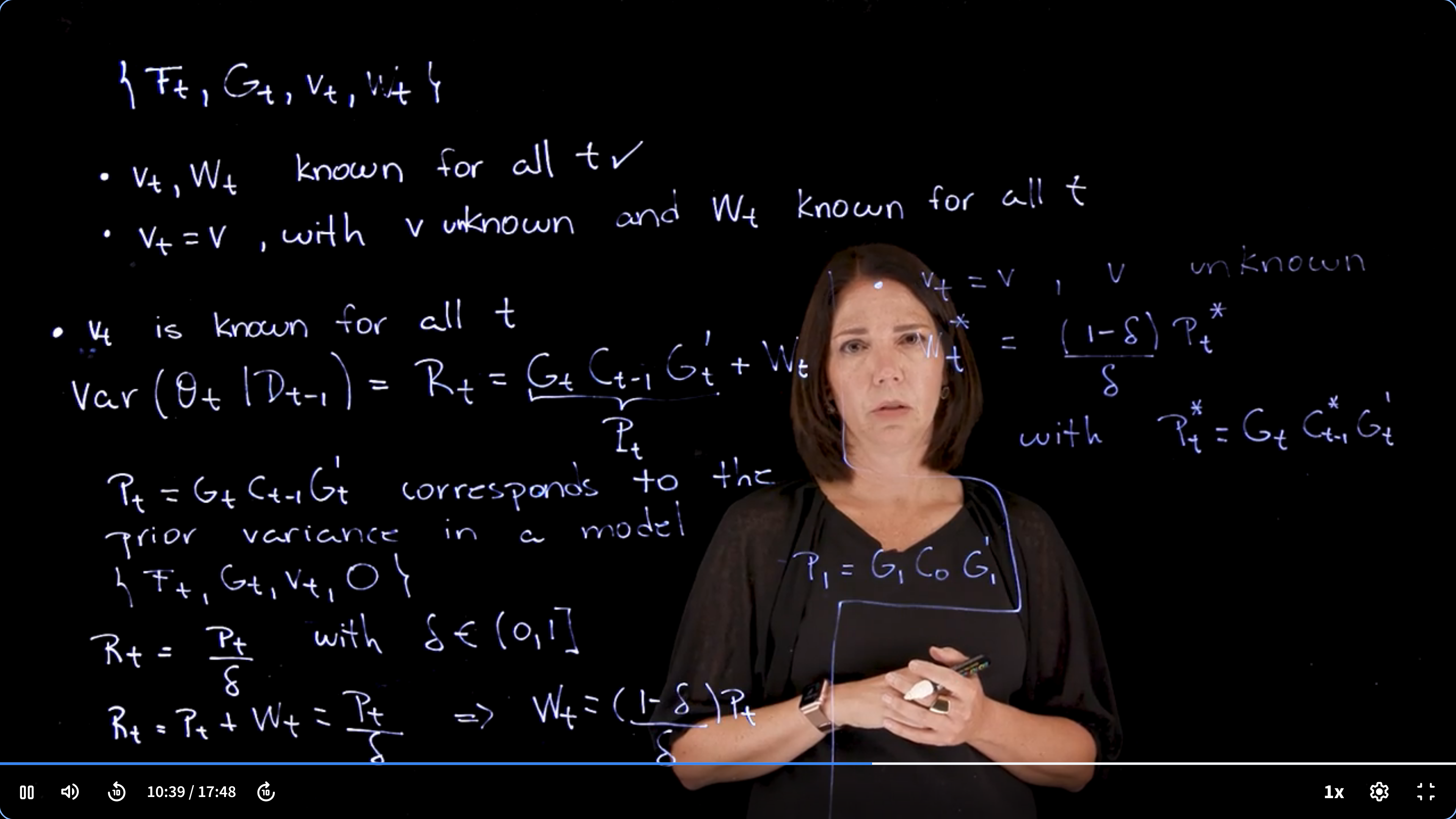
- So far we discussed $\{F_t,G_t,v_t,w_T\}$ with:
- $\underbrace{v_t}_{known}, \underbrace{w_t}_{known}$
- $v_t=\underbrace{v}_{unknown},\qquad \underbrace{w_t}_{known} \forall t$
- We move on to the case where:
- $v_t=\underbrace{v}_{known}, \forall t$ i.e. known observational variance
### Known observational variance with a discount factor \delta
$$
var(\theta_t\mid\mathcal{D}_t)=R_t=\underbrace{G_t C_{t-1}}_{P_t} G^\top_t + W_t
$$
- where $P_t = G_t C_{t-1}$ corresponds to the prior variance in the model with zero system variance i.e. $\{F_t,G_t,v_t,0\}$ with constant parameters that do not evolve over time!
- $R_t=\frac{P_t}{\delta} \qquad \delta \in (0,1]$
- $R_t P_t + W_t = \frac{P_t}{\delta} \implies W_t = \frac{1-\delta}{\delta}P_t$
we estimate
$$
P_1=G_1C_0G_1^T
$$
### Unknown constant observational variance with a discount factor \delta
$$
W_t^{*} = \frac{1-\delta}{\delta} P_t^{*}
$$
where:
$P_T^*=G_1C_0^*G_1^T$
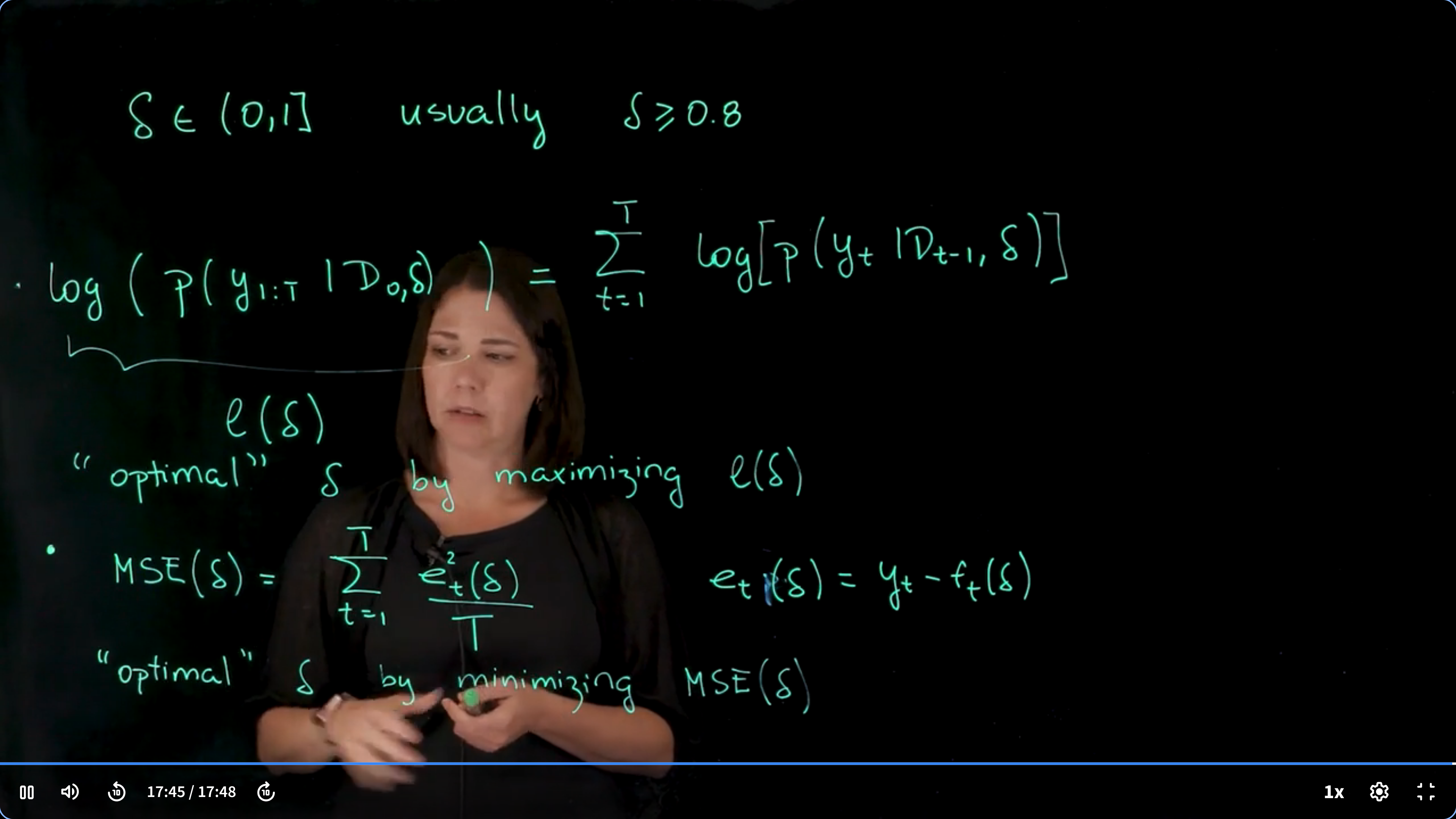
### Estimating $\delta$
$\delta\in(0,1] \text{ usually }\geq 0.8$
$$
\underbrace{\log(p(y_{1:T})\mid \mathcal{D}_0,\delta))}_{l(\delta)} = \sum log(p(y_t\mid \mathcal{D}_{t-1},\delta))
$$
we pick the optimal delta by maximizing $\mathcal{l}(\delta)$
$$
\textrm{MSE}(\delta) = \arg\max_{\delta} \mathcal{l}(\delta)) = \frac{1}{T}\sum_{t=1}^T (y_t - f_t(\delta))^2
$$
optimal $\delta$ is found by minimizing $MSE(\delta)$
but there are a number of methods to estimate $\delta$
we can have one delta for each component.
we can include it in the model and estimate it from the data.
::: {.callout-note collapse="true"}
## Video Transcript {.unnumbered}
{{< include transcripts/c4/04_week-4-normal-dynamic-linear-models-part-ii/02_bayesian-inference-in-the-ndlm-part-ii/03_specifying-the-system-covariance-matrix-via-discount-factors.en.txt >}}
:::
## NDLM, Unknown Observational Variance: Example :movie_camera:
This is a walk though of the R code in @lst-NDLM-unknown-variance
::: {.callout-note collapse="true"}
## Video Transcript {.unnumbered}
{{< include transcripts/c4/04_week-4-normal-dynamic-linear-models-part-ii/02_bayesian-inference-in-the-ndlm-part-ii/04_ndlm-unknown-observational-variance-example.en.txt >}}
:::
## code: NDLM, Unknown Observational Variance Example :spiral_notepad: $\mathcal{R}$
This code allows time-varying $F_t$, $G_t$ and $W_t$ matrices and assumes an unknown but constant $\nu$.
It also allows the user to specify $W_t$ using a discount factor $\delta \in (0,1]$ or assume $W_t$ known.
### Nile River Level Filtering Smoothing and Forecasting Example
```{r}
source('all_dlm_functions_unknown_v.R')
source('discountfactor_selection_functions.R')
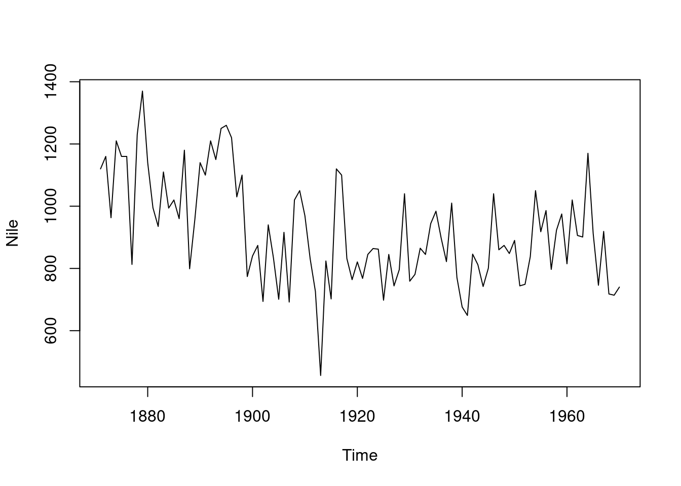
## Example: Nile River Level (in 10^8 m^3), 1871-1970
## Model: First order polynomial DLM
plot(Nile)
n=length(Nile) #n=100 observations
k=5
T=n-k
data_T=Nile[1:T]
test_data=Nile[(T+1):n]
data=list(yt = data_T)


## set up matrices for first order polynomial model
Ft=array(1, dim = c(1, 1, n))
Gt=array(1, dim = c(1, 1, n))
Wt_star=array(1, dim = c(1, 1, n))
m0=as.matrix(800)
C0_star=as.matrix(10)
n0=1
S0=10

## wrap up all matrices and initial values
matrices = set_up_dlm_matrices_unknown_v(Ft, Gt, Wt_star)
initial_states = set_up_initial_states_unknown_v(m0,
                                      C0_star, n0, S0)

## filtering
results_filtered = forward_filter_unknown_v(data, matrices,
                                            initial_states)
ci_filtered=get_credible_interval_unknown_v(results_filtered$mt,
                                    results_filtered$Ct,
                                     results_filtered$nt)

## smoothing
results_smoothed=backward_smoothing_unknown_v(data, matrices,
                                             results_filtered)
ci_smoothed=get_credible_interval_unknown_v(results_smoothed$mnt,
                                         results_smoothed$Cnt,
                                         results_filtered$nt[T])

## one-step ahead forecasting
results_forecast=forecast_function_unknown_v(results_filtered,
                                                k,  matrices)
ci_forecast=get_credible_interval_unknown_v(results_forecast$ft,
                                          results_forecast$Qt,
                                     results_filtered$nt[T])
```
```{r}
#| label: fig-NDLM-unknown-variance-nile-data
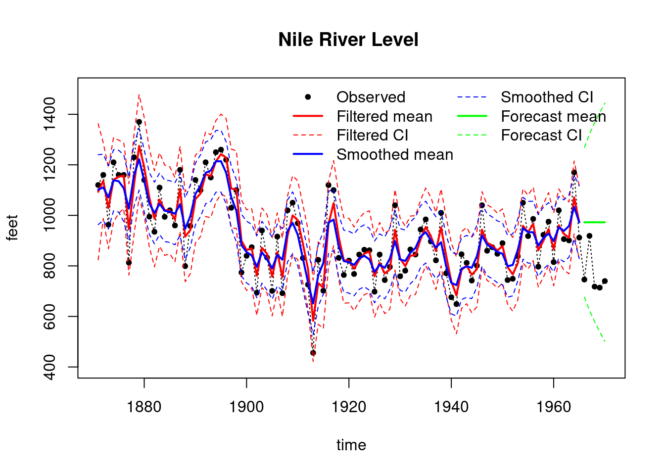
#| fig-cap: Nile River Level Filtering, Smoothing and Forecasting Results
## plot results
index=seq(1871, 1970, length.out = length(Nile))
index_filt=index[1:T]
index_forecast=index[(T+1):(T+k)]

plot(index, Nile, main = "Nile River Level ",type='l',
     xlab="time",ylab="feet",lty=3,ylim=c(400,1500))
points(index,Nile,pch=20)

lines(index_filt,results_filtered$mt, type='l', col='red',lwd=2)
lines(index_filt,ci_filtered[, 1], type='l', col='red', lty=2)
lines(index_filt,ci_filtered[, 2], type='l', col='red', lty=2)
lines(index_filt,results_smoothed$mnt, type='l', col='blue',lwd=2)
lines(index_filt, ci_smoothed[, 1], type='l', col='blue', lty=2)
lines(index_filt, ci_smoothed[, 2], type='l', col='blue', lty=2)

lines(index_forecast, results_forecast$ft, type='l',
      col='green',lwd=2)
lines(index_forecast, ci_forecast[, 1], type='l',
      col='green', lty=2)
lines(index_forecast, ci_forecast[, 2], type='l',
      col='green', lty=2)
legend("topright",
       legend = c("Observed", "Filtered mean", "Filtered CI",
                  "Smoothed mean", "Smoothed CI",
                  "Forecast mean", "Forecast CI"),
       col = c("black", "red", "red", "blue", "blue", "green", "green"),
       lty = c(NA, 1, 2, 1, 2, 1, 2),
       pch = c(20, NA, NA, NA, NA, NA, NA),
       lwd = c(NA, 2, 1, 2, 1, 2, 1),
       bty = "n",
       ncol = 2)
```
::: {.callout-note collapse="false"}
## Overthinking the Nile River Data {.unnumbered}
We use the Nile dataset throughout the course, despite the Nile data being notorious for having long term dependencies and being highly non-linear, which might present many challenges for the NDLM framework. c.f. the joint work of two giants [Benoit Mandelbrot](https://en.wikipedia.org/wiki/Benoit_Mandelbrot) and [Harold Edwin Hurst](https://en.wikipedia.org/wiki/Harold_Edwin_Hurst).
Which led to the development of the Hurst exponent and the [fractional Brownian motion](https://en.wikipedia.org/wiki/Fractional_Brownian_motion), i.e. fractional Gaussian noise and fractional ARIMA [ARFIMA](https://en.wikipedia.org/wiki/Autoregressive_fractionally_integrated_moving_average) which are more suitable for modeling the Nile data but not covered in this course.
Just a couple of concepts here:
In Fractional Brownian Motion (fBm) draws from the Normal need not be independent. With the concept of Hurst exponent $H$ which is a measure of the long-term memory of a time series. The Hurst exponent is defined as follows:
$$
\mathbb{E}[B_{H}(t)B_{H}(s)]={\tfrac {1}{2}}(|t|^{2H}+|s|^{2H}-|t-s|^{2H}),
$$ {#eq-fbm-autocovariance}
- where:
- $B_{H}(t)$ is the fractional Brownian motion, and
- $H$ is the Hurst exponent.
2. in ARFIMA, the autocovariance we allow the exponent of the lag $k$ to be a real number $d$ rather than an integer, i.e. we allow for fractional differencing via a formal binomial series expansion of the form:
$$\begin{array}{c} {\displaystyle {\begin{aligned}(1-B)^{d}&=\sum _{k=0}^{\infty }\;{d \choose k}\;(-B)^{k}\\&=\sum _{k=0}^{\infty }\;{\frac {\prod _{a=0}^{k-1}(d-a)\ (-B)^{k}}{k!}}\\&=1-dB+{\frac {d(d-1)}{2!}}B^{2}-\cdots \,.\end{aligned}}} \end{array}
$$ {#eq-ARFIMA}
:::
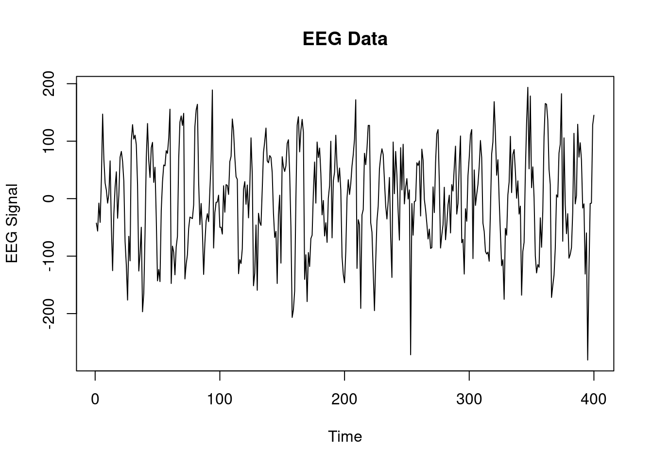
## Case Study EEG data :movie_camera: {#section-NDLM-eeg}
```{r}
### EEG example ##################
source('all_dlm_functions_unknown_v.R')
source('discountfactor_selection_functions.R')

eeg_data <- scan("data/eeg.txt")
length(eeg_data)
eeg_data_gh <- scan("data/eeg_gh.txt")
length(eeg_data_gh)
plot(eeg_data, type='l', main="EEG Data", xlab="Time", ylab="EEG Signal")
head(eeg_data)
head(eeg_data_gh)
T <- length(eeg_data)
data <- list(yt = eeg_data[])
```
::: {.callout-note collapse="true"}
## Video Transcript
{{< include transcripts/c4/04_week-4-normal-dynamic-linear-models-part-ii/03_case-studies/01_eeg-data.en.txt >}}
:::
## Case Study: Google Trends :movie_camera: {#section-NDLM-google-trends}
```{r}
```
::: {.callout-note collapse="true"}
## Video Transcript
{{< include transcripts/c4/04_week-4-normal-dynamic-linear-models-part-ii/03_case-studies/02_google-trends.en.txt >}}
:::