11.1 Inference example: frequentist
Example 11.1 (Two Coin Example) Suppose your brother has a coin that you know to be loaded so that it comes up heads 70% of the time. He then comes to you with some coin, you’re not sure which one and he wants to make a bet with you. Betting money that it’s going to come up heads.
You’re not sure if it’s the loaded coin or if it’s just a fair one. So he gives you a chance to flip it 5 times to check it out.
You flip it five times and get 2 heads and 3 tails.
We’ll start by defining the unknown parameter \theta, this is either that the coin is fair or it’s a loaded coin.
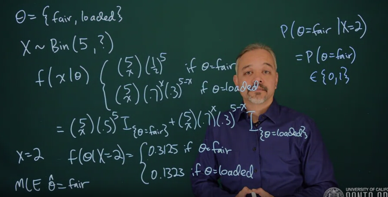
\theta = \{\text{fair},\ \text{loaded}\} \qquad \text{(parameter)} \tag{11.1}
we get to flip it five times but we do not know what kind of coin it is
X \sim Bin(5, \theta) \qquad \text{(model)} \tag{11.2}
each value of theta gives us a competing binomial likelihood:
f(x\ mid\theta) = \begin{cases} {5 \choose x}(\frac{1}{2})^5 & \theta = \text{fair} \\ {5 \choose x} (.7)^x (.3)^{5 - x} & \theta = \text{loaded} \end{cases} \qquad \text{(likelihood)} \tag{11.3}
We can also rewrite the likelihood f(x \mid \theta) using indicator functions
f(x\mid\theta) = {5\choose x}(.5)^5\mathbb{I}_{\{\theta= \text{fair}\}} + {5 \choose x}(.7)^x(.3)^{5 - x}\mathbb{I}_{\{\theta = \text{loaded}\}} \qquad \text{(likelihood)} \tag{11.4}
In this case, we observed that x = 2
f(\theta \mid x = 2) = \begin{cases} 0.3125 & \theta = \text{fair} \\ 0.1323 & \theta = \text{loaded} \end{cases} \qquad \text{(sub. x=2)} \tag{11.5}
\therefore \hat{\theta} = \text{fair} MLE \tag{11.6}
That’s a good point estimate, but then how do we answer the question, how sure are you?
This is not a question that’s easily answered in the frequentest paradigm. Another question is that we might like to know what is the probability that theta equals fair, give, we observe two heads.
\mathbb{P}r(\theta = \text{fair} \mid x = 2) = ? \tag{11.7}
In the frequentest paradigm, the coin is a physical quantity. It’s a fixed coin, and therefore it has a fixed probability of coining up heads. It is either the fair coin, or it’s the loaded coin.
\mathbb{P}r(\theta = \text{fair}) = \{0,1\}
11.2 Bayesian Approach to the Problem
An advantage of the Bayesian approach is that it allows you to easily incorporate prior information when you know something in advance of looking at the data. This is difficult to do under the frequentist paradigm.
In this case, we’re talking about your brother. You probably know him pretty well. So suppose you think that before you’ve looked at the coin, there’s a 60% probability that this is the loaded coin.
In this case, we put this into our prior. Our prior belief is that the probability the coin is loaded is 0.6. We can update our prior beliefs with the data to get our posterior beliefs, and we can do this using the Bayes theorem.
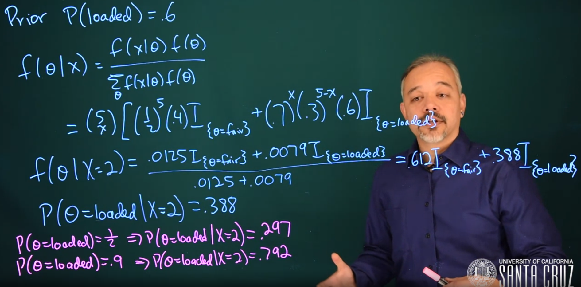
\begin{aligned} \mathbb{P}r(\text{loaded}) &= 0.6\ && \text{(prior)} \\ f(\theta \mid x) &= \frac{f(x \mid \theta)f(\theta)}{\sum_\theta{f(x \mid \theta)f(\theta)}} && \text{(Bayes)} \\ f(\theta\mid x=2)&= \frac{{5\choose x} \left [(\frac{1}{2})^5(1-0.6)\ \mathbb{I}_{(\theta = \text{fair})} + (.7)^x (.3)^{5-x}(.6)\ \mathbb{I}_{(\theta = \text{loaded})} \right] } {{5\choose x} \left [(\frac{1}{2})^5(.4) + (.7)^x (.3)^{5-x}(0.6) \right] }&& \text{(sub. x=2)} \\ &= \frac{0.0125\ \mathbb{I}_{(\theta = \text{fair})} + 0.0079\ \mathbb{I}_{(\theta = \text{loaded})} }{0.0125+0.0079}&& \text{(normalize)} \\ &= \textbf{0.612}\ \mathbb{I}_{(\theta=\text{fair})} + 0.388\ \mathbb{I}_{(\theta = \text{loaded})} && \text{(MLE)} \end{aligned} \tag{11.8}
As you can see in the calculation Equation 11.8, we have the likelihood times the prior in the numerator, and a normalizing constant in the denominator. When we divide the two, we’ll get an answer that adds up to 1. These numbers match exactly in this case because it’s a very simple problem.
This is a concept that we will revisit — what’s in the denominator here is always a normalizing constant.
\mathbb{P}r(\theta = loaded \mid x = 2) = 0.388
This here updates our beliefs after seeing some data about what the probability might be.
We can also examine what would happen under different choices of prior.
\mathbb{P}r(\theta = loaded) = \frac{1}{2} \implies \mathbb{P}r(\theta = loaded \mid x = 2) = 0.297
\mathbb{P}r(\theta = loaded) = 0.9 \implies \mathbb{P}r(\theta = loaded \mid x = 2) = 0.792
In this case, the Bayesian approach is inherently subjective. It represents your perspective, and this is an important part of the paradigm. If you have a different perspective, you will get different answers, and that’s okay. It’s all done in a mathematically vigorous framework, and it’s all mathematically consistent and coherent.
And in the end, we get interpretable results.
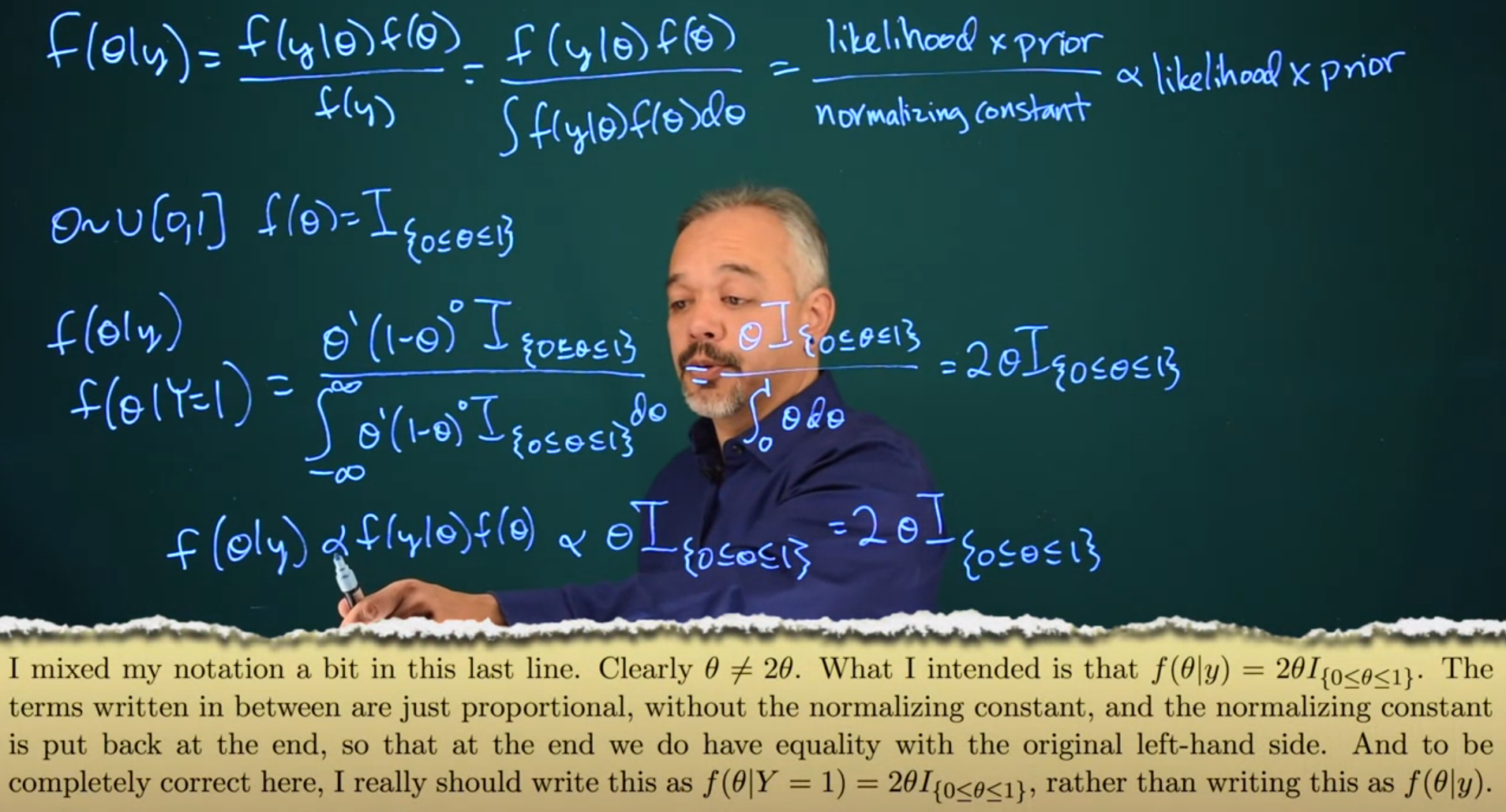
11.3 Continuous version of Bayes’ theorem
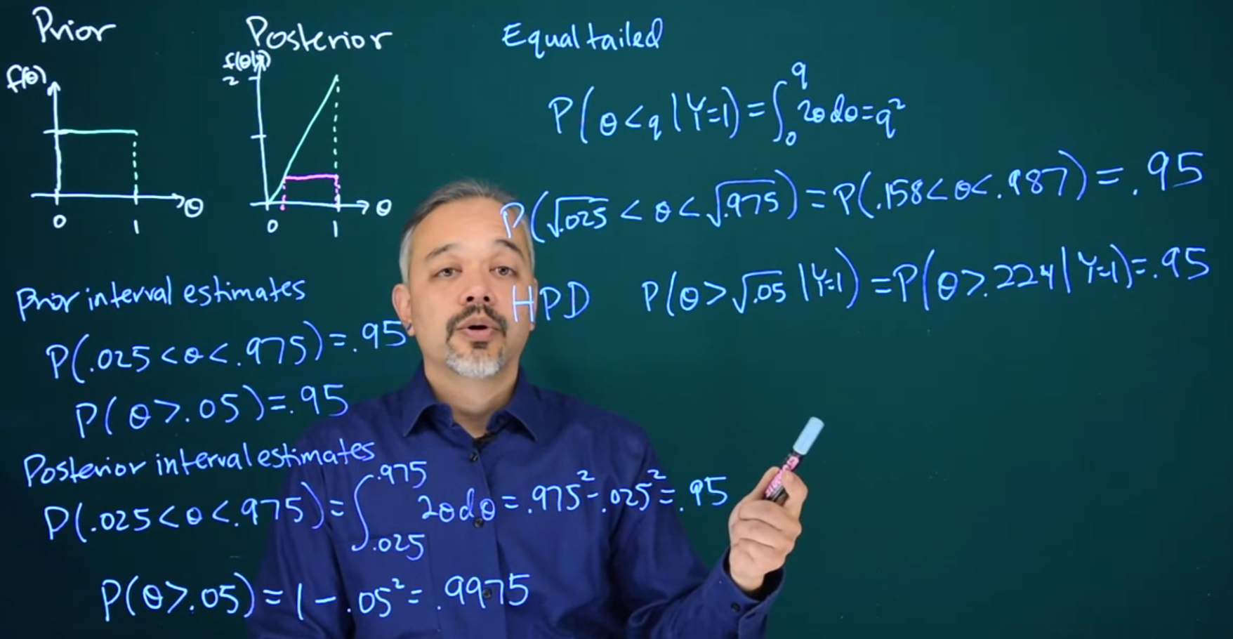
11.4 Posterior Intervals
11.5 Discussion CIs
- Frequentist confidence intervals have the interpretation that “If you were to repeat many times the process of collecting data and computing a 95% confidence interval, then on average about 95% of those intervals would contain the true parameter value; however, once you observe data and compute an interval the true value is either in the interval or it is not, but you can’t tell which.”
- Bayesian credible intervals have the interpretation that “Your posterior probability that the parameter is in a 95% credible interval is 95%.”
- Bayesian intervals treat their bounds as fixed and the estimated parameter as a random variable.
- Frequentist confidence intervals treat their bounds as random variables and the parameter as a fixed value.
11.5.1 Focusing on Bayesian / Frequentist paradigms
- A Frequentist CI might be preferred if:
- I had plenty of data to support a frequentist construction of frequentist CI and
- I was doing research and refining or refuting a result that has been established using frequentist hypothesis testing.
- I would want to show that for H_1 against some null hypothesis, H_0 the parameters have a certain p-value for some effect.
- Particularly when we are interested in the inference and are less interested in using the value of the parameter.
- I cannot justify introducing some subjective priors.
- A Bayesian CI might be better if:
- My dataset is too small.
- What I care about is the parameter’s value and less about hypothesis testing
- I need an estimate of uncertainty for the parameter for the inference it is used in.
- I had subjective reasons to introduce a prior:
- I know about constraints
- I have access to expert knowledge
- I wish to introduce pooling between groups, to share information for reducing uncertainty.
- My results are in a Bayesian-oriented domain.
11.5.2 Focusing on the CI choices
Let’s point out that this is what we call a loaded question, as it has a bias against the frequentist approach by stating one of its shortcomings when it is still possible to get a point estimate for the parameter and compare it to the CI. Typically one will have already done it say using regression before considering the CI.
Next, we have all the standard reasons for choosing between the Frequentist and the Bayesian paradigms. I could list them but I don’t think that is the real point of this question, but rather what would we prefer if both were viable options and why?
CIs are primarily a tool for understanding uncertainties about parameters that encode effects. In the parametric Bayesian approach we are learning the distribution of our parameters so they have uncertainties baked into them. In the Frequentist approach, we look for the least squares point estimates for our parameters and consider using the CI to approximate the long-run uncertainty due to sampling.
Frequentist CI might be preferable if I am worried about Aletoric uncertainty due to sampling i.e. to what degree can I be certain my experimental outcomes are not due to chance? I would feel this way since I am a classical physicist or a botanist studying a predominately deterministic effect and I see errors in estimating the parameters as artifacts of sampling that can be made smaller till the parameters will converge with the true population statistics and the error will become vanishingly small.
Given that I did my best to get a good data sample I just need to check how sure to decide the cardinal question do I publish or do I perish? I need to decide that the result is due to the effect and not due to some conspiracy bad samples.
Bayesian CIs are just a result of using Bayesian analysis which is a requirement to investigate what are predominately random effects that are the domain of quantum physicists, an ecologist, or a geneticist. Since almost everything I study is predominantly random and I need random variables and Bayes law to get to my results. I also need to report confidence intervals for my work when I publish - but if one is a Bayesian, one will use a Bayesian credible interval?