Where we used a trick of recognizing the denominator as a Beta distribution (Equation C.7) we then manipulate it to take the exact form of Beta. We can then cancel it since the Beta density integrates to 1, we can simplify this as From here we can see that the posterior follows a Beta distribution
\theta \mid y \sim \mathrm{Beta}\left (\sum{y_i} + 1, n - \sum{y_i} + 1 \right )
Figure 16.2: R.A. Fisher
TipHistorical Note on Sir Ronald Aylmer Fisher FRS
R.A. Fisher’s objection to the Bayesian approach is that “The theory of inverse probability is founded upon an error, and must be wholly rejected”(Fisher 1925) was specifically referring to this example of a”Binomial with a Uniform prior”. The gist of it is that the posterior depends on the parametrization of the prior.(Aldrich 2008). Sir Harold Jeffreys FRS who corresponded with Fisher went on to develop his eponymous priors which were invariant to reparametrization. Which we will consider in Section 25.2
16.2 Conjugate Priors
Figure 16.3: Conjugate Priors
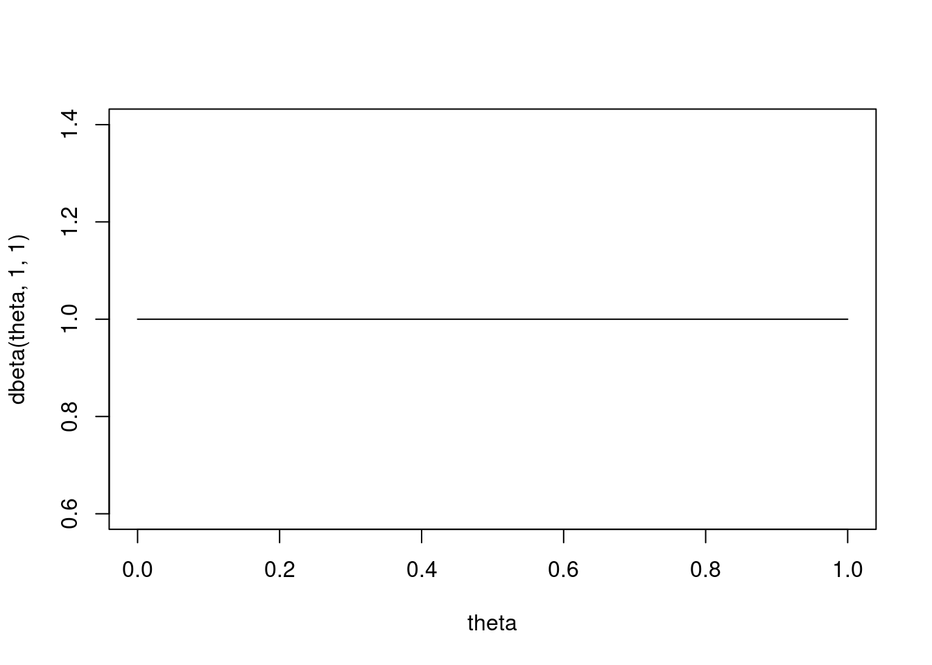
The Uniform distribution is \mathrm{Beta}(1, 1)
Any beta distribution is conjugate for the Bernoulli distribution. Any beta prior will give a beta posterior.
\theta \mid y \sim \mathrm{Beta}(\alpha + \sum{y_i}, \beta + n - \sum{y_i})
When \alpha and \beta are one like in the uniform distribution, then we get the same result as earlier.
This whole process where we choose a particular form of prior that works with a likelihood is called using a conjugate family.
A family of distributions is referred to as conjugate if when you use a member of that family as a prior, you get another member of that family as your posterior.
The beta distribution is conjugate for the Bernoulli distribution. It’s also conjugate for the binomial distribution. The only difference in the binomial likelihood is that there is a combinatorics term. Since that does not depend on \theta, we get the same posterior.
We often use conjugate priors because they make life much simpler, sticking to conjugate families allows us to get closed-form solutions easily.
If the family is flexible enough, then you can find a member of that family that closely represents your beliefs.
the Uniform distribution can be written as the \mathrm{Beta}(1,1) prior.
Any Beta prior will result in a Beta posterior.
Beta is conjugate for Binomial and for Bernoulli
16.3 Posterior mean and effective sample size
Figure 16.4: Effective Sample Size
Returning to the Beta posterior model it is clear how both the prior and the data contribute to the posterior.
For a prior \mathrm{Beta}(\alpha,\beta) we can say that the effective sample size of the prior is
\alpha + \beta \qquad \text {(ESS)}
\tag{16.1}
Recall that the expected value or mean of a Beta distribution is \frac{\alpha}{\alpha + \beta}
i.e. The posterior mean is a weighted average of the prior mean and the data mean.
This effective sample size gives you an idea of how much data you would need to make sure that your prior does not have much influence on your posterior.
If \alpha + \beta is small compared to n then the posterior will largely just be driven by the data. If \alpha + \beta is large relative to n then the posterior will be largely driven by the prior.
We can make a 95% credible interval using our posterior distribution for \theta . We can find an interval that has 95 \% probability of containing \theta.
Using Bayesian Statistics we can do sequential analysis by doing a sequential update every time we get new data. We can get a new posterior, and we just use our previous Posterior as a Prior for doing another update using Bayes’ theorem.
Figure 16.5: ESS algorithms
for a Beta prior, its effective sample size is a + b
if n >> \alpha+\beta the posterior will be predominantly determined by the prior
if n << \alpha+\beta the posterior will be predominantly determined by the data
the idea of an effective sample size of the prior is a useful concept to work with.
Suppose we are interested in global temperatures, and that we have a summary measure that represents the average global temperature for each year. Now we could ask “What is the probability that next year will have a higher average global temperature than this year?” What would be your choice of prior and why? Be specific about the distribution and its parameters. You may use any other information that you want to bring into this problem.
TipResponse
It is possible to get historical estimates using:
Meteorological and satellites for the last 200 years. Figure 16.6
Deep sea sediment oxygen 18 isotope fractation for the last 5 million years. Figure 16.8
or yearly temperature data from 1850 till today based on meteorological readings. We can also consider Greenland ice core data covering 800,000 years.
One simple way is to model the yearly temperature as a random walk
i.e. Each year is a Bernoulli trial where success is the temperature getting warmer. We can then use the historical data since 1800 to estimate theta the probability that we get warmer.
I suppose we can use a Binomial prior with parameters for alpha the count of years the temperature increased and N for the total number of years and p the probability the a given year is hotter than the previous.
16.4 Data Analysis Example in R
Suppose we’re giving two students a multiple-choice exam with 40 questions, where each question has four choices. We don’t know how much the students have studied for this exam, but we think that they’ll do better than just guessing randomly
What are the parameters of interest?
The parameters of interests are \theta_1 = true the probability that the first student will answer a question correctly, \theta_2 = true the probability that the second student will answer a question correctly.
What is our likelihood?
The likelihood is \mathrm{Binomial}(40, \theta) if we assume that each question is independent and that the probability a student gets each question right is the same for all questions for that student.
What prior should we use?
The Conjugate Prior is a Beta Distribution. We can plot the density with dbeta
theta =seq(from =0, to =1, by =0.1)# Uniformplot(theta, dbeta(theta, 1, 1), type ='l')
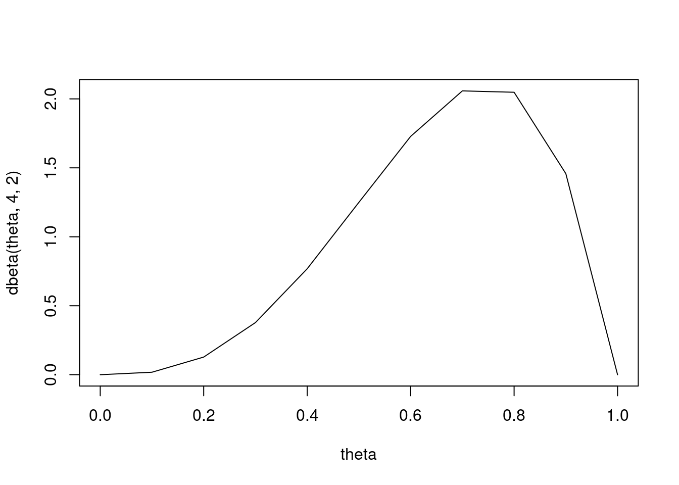
# Prior mean 2/3plot(theta, dbeta(theta, 4, 2), type ='l')
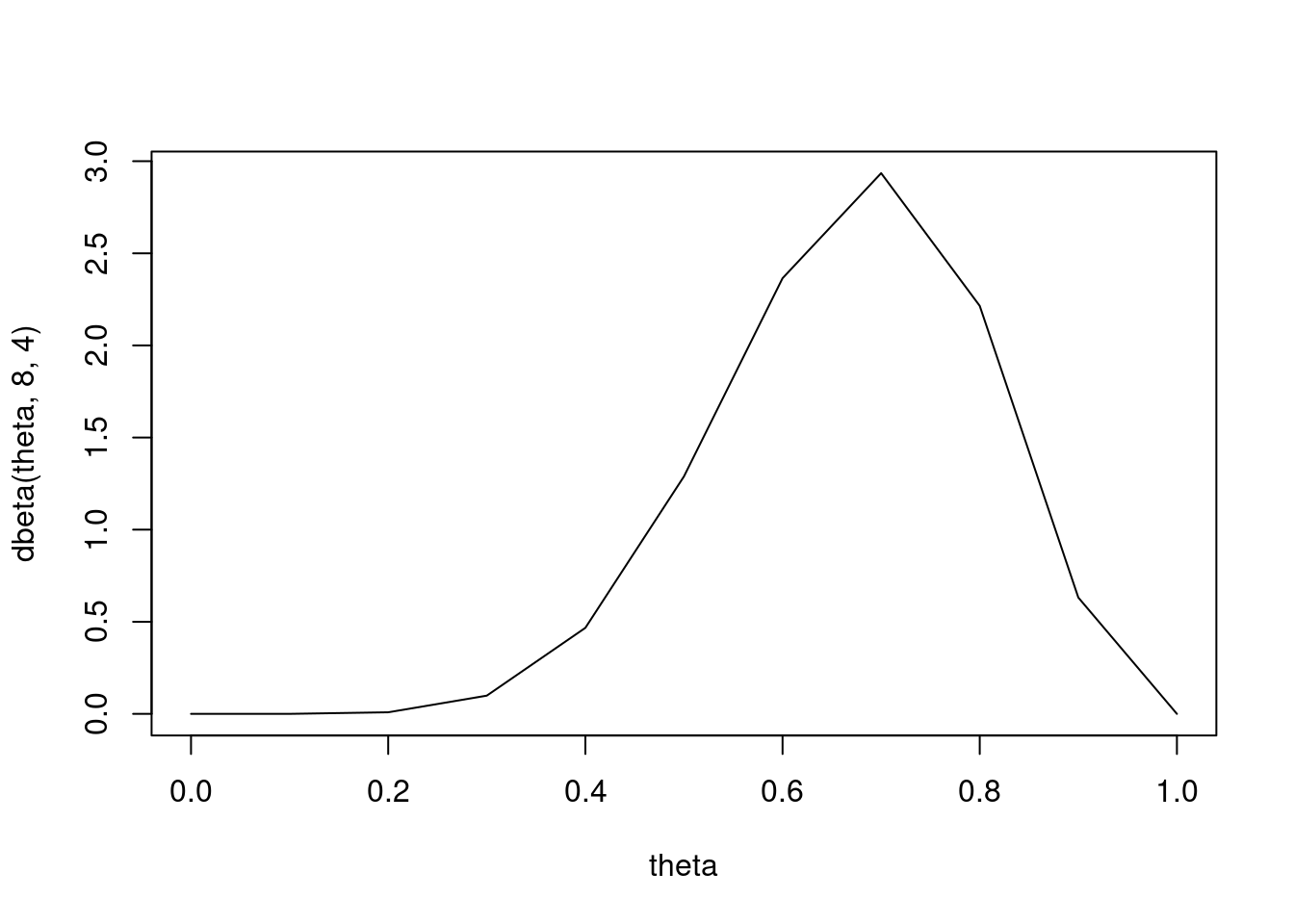
# Prior mean 2/3 but higher effect size (more concentrated at mean)plot(theta, dbeta(theta, 8, 4), type ='l')
What are the prior probabilities \mathbb{P}r(\theta > 0.25)? \mathbb{P}r(\theta > 0.5)? \mathbb{P}r(\theta > 0.8)?
1-pbeta(0.25, 8, 4)
[1] 0.9988117
#[1] 0.9981171-pbeta(0.5, 8, 4)
[1] 0.8867188
#[1] 0.88671881-pbeta(0.8, 8, 4)
[1] 0.1611392
#[1] 0.16113392
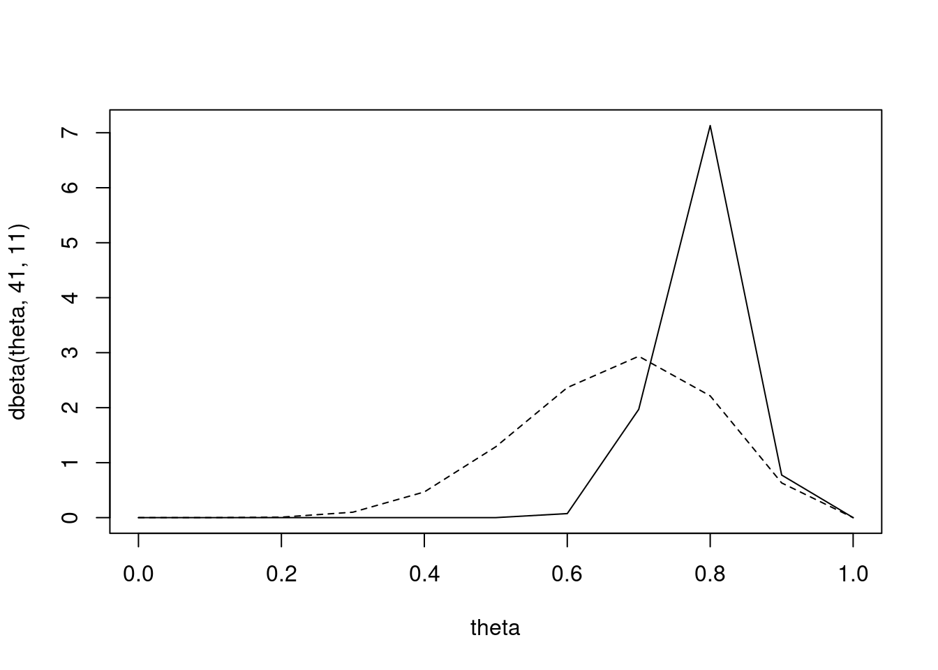
Suppose the first student gets 33 questions right. What is the posterior distribution for \theta_1 ? \mathbb{P}r(\theta > 0.25) ? \mathbb{P}r(\theta > 0.5) ? \mathbb{P}r(\theta > 0.8) ? What is the 95% posterior credible interval for \theta_1?
With a posterior mean of \frac{41}{41+11} = \frac{41}{52}
We can plot the posterior distribution with the prior
plot(theta, dbeta(theta, 41, 11), type ='l')lines(theta, dbeta(theta, 8 ,4), lty =2) #Dashed line for prior
Posterior probabilities
1-pbeta(0.25, 41, 11)
[1] 1
#[1] 11-pbeta(0.5, 41, 11)
[1] 0.9999926
#[1] 0.99999261-pbeta(0.8, 41, 11)
[1] 0.4444044
#[1] 0.4444044
Equal-tailed 95% credible interval
qbeta(0.025, 41, 11)
[1] 0.6688426
#[1] 0.6688426qbeta(0.975, 41, 11)
[1] 0.8871094
#[1] 0.8871094
95% confidence that \theta_1 is between 0.67 and 0.89
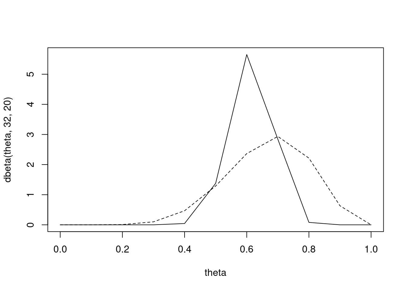
Suppose the second student gets 24 questions right. What is the posterior distribution for \theta_2? \mathbb{P}r(\theta > 0.25)? \mathbb{P}r(\theta > 0.5)? \mathbb{P}r(\theta > 0.8)? What is the 95% posterior credible interval for \theta_2
Fisher, R. A. 1925. Statistical Methods for Research Workers. 1st ed. Edinburgh Oliver & Boyd.
Morita, Satoshi, Peter F Thall, and Peter Müller. 2008. “Determining the Effective Sample Size of a Parametric Prior.”Biometrics 64 (2): 595–602.
Wiesenfarth, Manuel, and Silvia Calderazzo. 2020. “Quantification of Prior Impact in Terms of Effective Current Sample Size.”Biometrics 76 (1): 326–36. https://doi.org/https://doi.org/10.1111/biom.13124.
Source Code
---title: "M3L7 - Binomial Data"subtitle: "Bayesian Statistics: From Concept to Data Analysis"subject: "Bayesian Statistics"description: "Outline of probability"categories: - Bayesian Statisticskeywords: - Binomial Data - Binomial Distribution - Bernoulli Distribution - Beta Distribution---## Bernoulli/Binomial likelihood with a uniform prior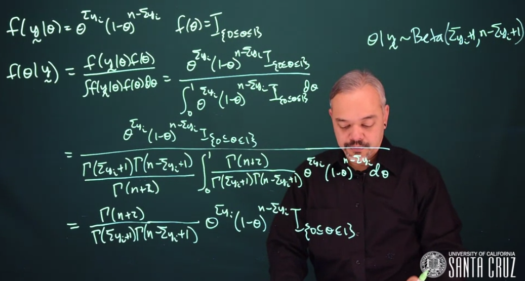{#fig-binomial-likelihood-uniform-prior .column-margin width="53mm"}When we use a uniform prior for a Bernoulli likelihood, we get a beta posterior.The Bernoulli likelihood of $\vec Y \mid \theta$ is$${\color{green}f(\vec Y \mid \theta) = {\theta^{\sum{y_i}}(1-\theta)^{n - \sum{y_i}}}} \qquad \text{Bernoulli Likelihood}$$Our prior for $\theta$ is just a Uniform distribution$${\color{red}f(\theta) = I_{\{0 \le \theta \le 1\}} }\qquad \text {Uniform prior}$$Thus our posterior for $\theta$ is$$\begin{aligned}f(\theta \mid y) & = \frac{f(y \mid \theta) f(\theta)}{\int f(y \mid \theta)f(\theta) \, d\theta} & \text{Bayes law} \\& = \frac{\theta^{\sum{y_i}} (1 - \theta)^{n - \sum{y_i}} \mathbb{I}_{\{0 \le \theta \le 1\}}}{\int_0^1 \theta^{\sum{y_i}}(1 - \theta)^{n - \sum{y_i}} \mathbb{I}_{\{0 \le \theta \le 1\}} \, d\theta} & \text{subst. Likelihood \& Prior} \\& = \frac{\theta^{\sum{y_i}} (1-\theta)^{n - \sum{y_i}} \mathbb{I}_{\{0 \le \theta \le 1\}}}{\frac{\Gamma(\sum{y_i} + 1)\Gamma(n - \sum{y_i} + 1)}{\Gamma(n + 2)} \cancel{\int_0^1 \frac{\Gamma(n + 2)}{\Gamma(\sum{y_i} + 1) \Gamma(n - \sum{y_i} + 1)} \theta^{\sum{y_i}} (1 - \theta)^{n - \sum{y_i}} \, d\theta}} & \text{Beta PDF integrates to 1} \\& = \frac{\Gamma(n + 2)}{\Gamma(\sum{y_i}+ 1) \Gamma(n - \sum{y_i}+ 1)} \theta^{\sum{y_i}}(1 - \theta)^{n - \sum{y_i}} \mathbb{I}_{\{0 \le \theta \le 1\}} & \text{simplifying} \\& = \mathrm{Beta} \left (\sum{y_i} + 1, n - \sum{y_i} + 1 \right )\end{aligned}$$Where we used a trick of recognizing the denominator as a *Beta distribution* (@eq-beta-pdf) we then manipulate it to take the exact form of *Beta*. We can then cancel it since the *Beta density* integrates to $1$, we can simplify this as From here we can see that the posterior follows a *Beta distribution*$$\theta \mid y \sim \mathrm{Beta}\left (\sum{y_i} + 1, n - \sum{y_i} + 1 \right )$$\index{Fisher, R.A.}\index{{Fisher, Ronald Aylmer}|see{Fisher, R.A.}}\index{{Fisher, Ronald}|see{Fisher, R.A.}}\index{Jeffreys, Harold}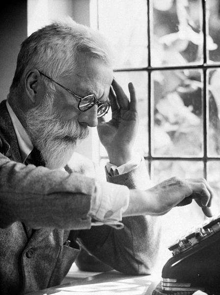{#fig-rafisher .column-margin width="53mm"} ::: {.callout-tip}## Historical Note on Sir Ronald Aylmer Fisher FRSR.A. Fisher's objection to the Bayesian approach is that "The theory of inverse probability **is founded upon an error, and must be wholly rejected"** [@Fisher1925Statistical] was specifically referring to this example of a "Binomial with a Uniform prior". The gist of it is that the posterior depends on the parametrization of the prior.[@Aldrich2008Fisher]. Sir Harold Jeffreys FRS who corresponded with Fisher went on to develop his eponymous priors which were invariant to reparametrization. Which we will consider in [@sec-jeffreys-prior]:::## Conjugate Priors {#sec-conjugate-beta-priors}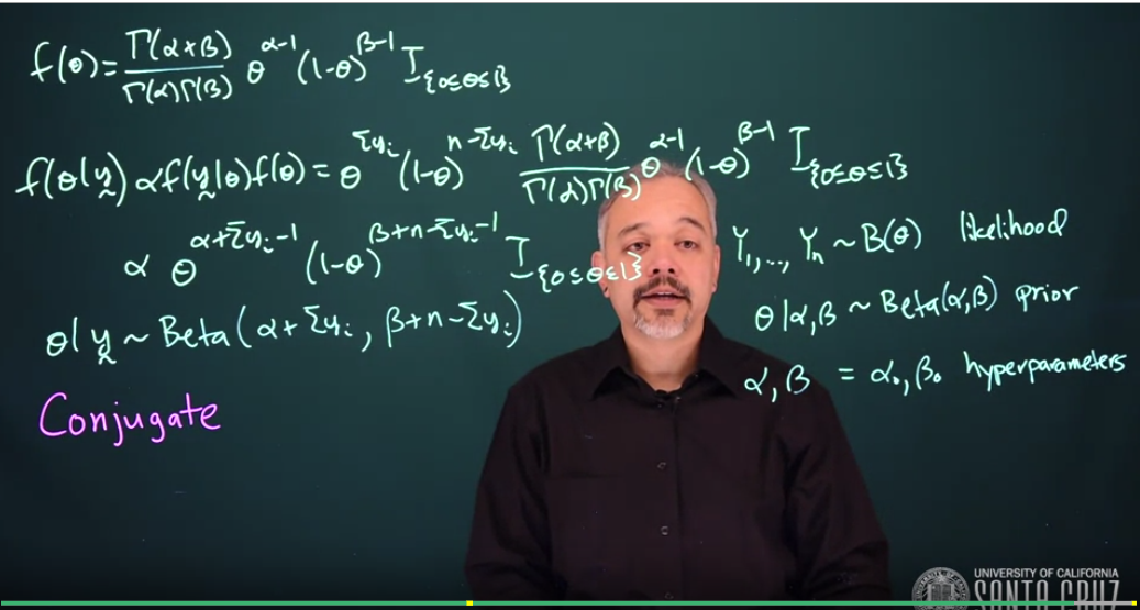{#fig-s03-conjugate-priors .column-margin width="53mm"}The Uniform distribution is $\mathrm{Beta}(1, 1)$Any beta distribution is conjugate for the *Bernoulli distribution*. Any *beta prior* will give a *beta posterior*.$$f(\theta) = \frac{\Gamma(\alpha + \beta)}{\Gamma(\alpha)\Gamma(\beta)}\theta^{\alpha - 1}(1-\theta)^{\beta -1}\mathbb{I}_{\{\theta \le \theta \le 1\}}$$ $$f(\theta \mid y) \propto f(y \mid \theta)f(\theta) = \theta^{\sum{y_i}}(1-\theta)^{n - \sum{y_i}}\frac{\Gamma(\alpha + \beta)}{\Gamma(\alpha)\Gamma(\beta)}\theta^{\alpha - 1}(1 - \theta)^{\beta - 1}\mathbb{I}_{\{\theta \le \theta \le 1\}}$$$$f(y \mid\theta)f(\theta) \propto \theta^{\alpha + \sum{y_i}-1}(1-\theta)^{\beta + n - \sum{y_i} - 1}$$Thus we see that this is a beta distribution$$\theta \mid y \sim \mathrm{Beta}(\alpha + \sum{y_i}, \beta + n - \sum{y_i})$$When $\alpha$ and $\beta$ are one like in the uniform distribution, then we get the same result as earlier.This whole process where we choose a particular form of prior that works with a likelihood is called using a conjugate family.A family of distributions is referred to as conjugate if when you use a member of that family as a prior, you get another member of that family as your posterior.The beta distribution is conjugate for the Bernoulli distribution. It's also conjugate for the binomial distribution. The only difference in the binomial likelihood is that there is a combinatorics term. Since that does not depend on $\theta$, we get the same posterior.\index{prior!conjugate}We often use conjugate priors because they make life much simpler, sticking to conjugate families allows us to get closed-form solutions easily.If the family is flexible enough, then you can find a member of that family that closely represents your beliefs.- the Uniform distribution can be written as the $\mathrm{Beta}(1,1)$ prior.- Any *Beta prior* will result in a *Beta posterior*.- *Beta* is conjugate for Binomial and for Bernoulli## Posterior mean and effective sample size {#sec-effective-sample-size}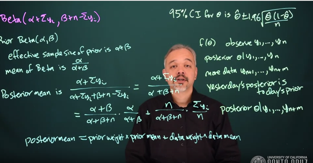{#fig-s04-effective-sample-size .column-margin width="53mm"}Returning to the *Beta* posterior model it is clear how both the prior and the data contribute to the posterior.For a prior $\mathrm{Beta}(\alpha,\beta)$ we can say that the **effective sample size** of the prior is $$\alpha + \beta \qquad \text {(ESS)}$$ {#eq-beta-ess}Recall that the expected value or mean of a *Beta* distribution is $\frac{\alpha}{\alpha + \beta}$Therefore we can derive the posterior mean as$$\begin{aligned} posterior_{mean} &= \frac{\alpha + \sum{y_i}}{\alpha + \sum{y_i}+\beta + n - \sum{y_i}}\\ &= \frac{\alpha+\sum{y_i}}{\alpha + \beta + n}\\ &= \frac{\alpha + \beta}{\alpha + \beta + n}\frac{\alpha}{\alpha + \beta} + \frac{n}{\alpha + \beta + n}\frac{\sum{y_i}}{n}\\ &= (\text{prior weight} \times \text{prior mean}) + (\text{data weight} \times \text{data mean})\end{aligned}$$ {#eq-beta-posterior-mean-derivation}i.e. The **posterior mean** is a weighted average of the **prior mean** and the **data mean**.\index{MCMC!effective sample size}This effective sample size gives you an idea of how much data you would need to make sure that your prior does not have much influence on your posterior.If $\alpha + \beta$ is small compared to $n$ then the posterior will largely just be driven by the data. If $\alpha + \beta$ is large relative to $n$ then the posterior will be largely driven by the prior.We can make a 95% credible interval using our posterior distribution for $\theta$ . We can find an interval that has $95 \%$ probability of containing $\theta$.\index{sequential analysis}Using Bayesian Statistics we can do *sequential analysis* by doing a sequential update every time we get new data. We can get a new posterior, and we just use our previous Posterior as a Prior for doing another update using Bayes' theorem.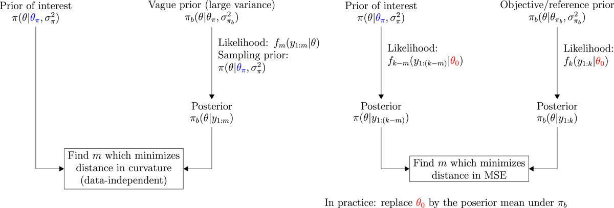{#fig-ess-paper .column-margin width="53mm"}- for a *Beta prior*, its *effective sample size* is $a + b$- if $n >> \alpha+\beta$ the posterior will be predominantly determined by the prior- if $n << \alpha+\beta$ the posterior will be predominantly determined by the data- the idea of an effective sample size of the prior is a useful concept to work with.- [@Wiesenfarth2020Quantification] - Effective Sample Size (ESS) - Effective Current Sample size (ECSS) - with [@morita2008determining] on the left and ECSS on the right{#fig-200-year-meterological .column-margin width="53mm"}{#fig-800K-year-ice-core .column-margin width="53mm"}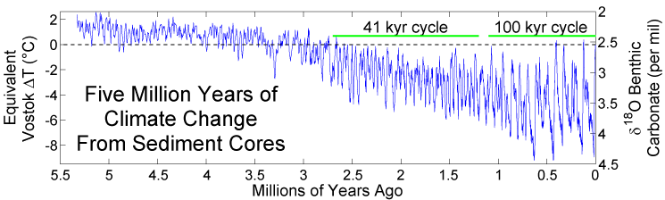{#fig-five-year-deep-sea .column-margin width="53mm"}::: {#exr-prior-elicitation}## Discussion on Prior elicitation> Suppose we are interested in global temperatures, and that we have a summary measure that represents the average global temperature for each year. > Now we could ask "What is the probability that next year will have a higher average global temperature than this year?" > What would be your choice of prior and why? > Be specific about the distribution and its parameters. > You may use any other information that you want to bring into this problem.:::::: {.callout-tip collapse="true"}## Response {.unnumbered}It is possible to get historical estimates using:- Meteorological and satellites for the last 200 years. @fig-200-year-meterological- Ice cores for the last 800,000 years @fig-800K-year-ice-core- Deep sea sediment oxygen 18 isotope fractation for the last 5 million years. @fig-five-year-deep-seaor yearly temperature data from 1850 till today based on meteorological readings. We can also consider Greenland ice core data covering 800,000 years.One simple way is to model the yearly temperature as a random walki.e. Each year is a Bernoulli trial where success is the temperature getting warmer. We can then use the historical data since 1800 to estimate theta the probability that we get warmer.I suppose we can use a Binomial prior with parameters for alpha the count of years the temperature increased and N for the total number of years and p the probability the a given year is hotter than the previous.:::## Data Analysis Example in RSuppose we're giving two students a multiple-choice exam with 40 questions, where each question has four choices. We don't know how much the students have studied for this exam, but we think that they'll do better than just guessing randomly1. What are the parameters of interest?The parameters of interests are $\theta_1 = true$ the probability that the first student will answer a question correctly, $\theta_2 = true$ the probability that the second student will answer a question correctly.2. What is our likelihood?The likelihood is $\mathrm{Binomial}(40, \theta)$ if we assume that each question is independent and that the probability a student gets each question right is the same for all questions for that student.3. What prior should we use?The **Conjugate Prior** is a **Beta Distribution**. We can plot the density with `dbeta````{R}#| label: C1-L07-1theta =seq(from =0, to =1, by =0.1)# Uniformplot(theta, dbeta(theta, 1, 1), type ='l')# Prior mean 2/3plot(theta, dbeta(theta, 4, 2), type ='l')# Prior mean 2/3 but higher effect size (more concentrated at mean)plot(theta, dbeta(theta, 8, 4), type ='l')```4. What are the prior probabilities $\mathbb{P}r(\theta > 0.25)$? $\mathbb{P}r(\theta > 0.5)$? $\mathbb{P}r(\theta > 0.8)$?```{R}#| label: C1-L07-21-pbeta(0.25, 8, 4)#[1] 0.9981171-pbeta(0.5, 8, 4)#[1] 0.88671881-pbeta(0.8, 8, 4)#[1] 0.16113392```5. Suppose the first student gets 33 questions right. What is the posterior distribution for $\theta_1$ ? $\mathbb{P}r(\theta > 0.25)$ ? $\mathbb{P}r(\theta > 0.5)$ ? $\mathbb{P}r(\theta > 0.8)$ ? What is the 95% posterior credible interval for $\theta_1$? $$\text{Posterior} \sim \mathrm{Beta}(8 + 33, 4 + 40 - 33) = \mathrm{Beta}(41, 11)$$With a posterior mean of $\frac{41}{41+11} = \frac{41}{52}$We can plot the posterior distribution with the prior```{R}#| label: C1-L07-3plot(theta, dbeta(theta, 41, 11), type ='l')lines(theta, dbeta(theta, 8 ,4), lty =2) #Dashed line for prior```Posterior probabilities```{R}#| label: C1-L07-41-pbeta(0.25, 41, 11)#[1] 11-pbeta(0.5, 41, 11)#[1] 0.99999261-pbeta(0.8, 41, 11)#[1] 0.4444044```Equal-tailed 95% credible interval```{R}#| label: C1-L07-5qbeta(0.025, 41, 11)#[1] 0.6688426qbeta(0.975, 41, 11)#[1] 0.8871094```95% confidence that $\theta_1$ is between 0.67 and 0.896. Suppose the second student gets 24 questions right. What is the posterior distribution for $\theta_2$? $\mathbb{P}r(\theta > 0.25)$? $\mathbb{P}r(\theta > 0.5)$? $\mathbb{P}r(\theta > 0.8)$? What is the 95% posterior credible interval for $\theta_2$$$\text{Posterior} \sim \mathrm{Beta}(8 + 24, 4 + 40 - 24) = \mathrm{Beta}(32, 20)$$With a posterior mean of $\frac{32}{32+20} = \frac{32}{52}$We can plot the posterior distribution with the prior```{R}#| label: C1-L07-6plot(theta, dbeta(theta, 32, 20), type ='l')lines(theta, dbeta(theta, 8 ,4), lty =2) #Dashed line for prior```Posterior probabilities```{R}#| label: C1-L07-71-pbeta(0.25, 32, 20)#[1] 11-pbeta(0.5, 32, 20)#[1] 0.95404271-pbeta(0.8, 32, 20)#[1] 0.00124819```Equal-tailed 95% credible interval```{R}#| label: C1-L07-8qbeta(0.025, 32, 20)#[1] 0.4808022qbeta(0.975, 32, 20)#[1] 0.7415564```95% confidence that $\theta_1$ is between 0.48 and 0.747. What is the posterior probability that $\theta_1 > \theta_2$?i.e., that the first student has a better chance of getting a question right than the second student?Estimate by simulation: draw 1,000 samples from each and see how often we observe $\theta_1 > \theta_2$```{R}#| label: C1-L07-9theta1 =rbeta(100000, 41, 11)theta2 =rbeta(100000, 32, 20)mean(theta1 > theta2)#[1] 0.975```