---
title: "Poisson regression - M4L10"
subtitle: "Bayesian Statistics: Techniques and Models"
description: "An overview of Poisson regression in the context of Bayesian statistics."
categories:
- Monte Carlo Estimation
keywords:
- Poisson regression
- Bayesian statistics
- R programming
- statistical modeling
- count data
- Poisson distribution
- over dispersion
- zero-inflated models
---
\index{regression!Poisson}
\index{distribution!negative binomial}
\index{distribution!Poisson}
Poisson regression is the preferred method to handle count data where the response is positive values but includes zeroes.
The gist of this method is that We use a log transform link function on the regressors but not on the response which allows the response to be zero valued which correspond to zero counts.
One limit of this approach mentioned below is that the Poisson takes one parameter $\lambda$ for both its expected value and its variance.
We look give a deeper solution to this problem in the next course on mixture models, however in this course we will consider more restricted cases where we
extend the Poisson regression with the **Negative Binomial Distribution**
which allows us to model over-dispersed data.
::: {.callout-note}
#### Overdispersion {#sec-overdispersion}
\index{overdispersion}
\index{regression!Poisson}
In cases where the variance needs to be a separate feature of the model we can use an alternative model with additional free parameters may provide a better fit. In this case of count data, a Poisson mixture model like the Negative Binomial Distribution can be posited instead, in which the mean of the Poisson distribution can itself be thought of as a random variable drawn -- from the Gamma distribution thereby introducing an additional free parameter
We don't see the case of over-dispersion in this course but the next course is on mixture models.
:::
## Introduction to Poisson regression {#sec-introduction-to-poisson-regression}
\index{regression!Poisson}
{#fig-intro-poisson-regression .column-margin width="53mm" group="slides"}
We now have experience fitting regression models when the response is continuous, and when it is binary.
What about when we have count data?
We could fit a linear normal regression, but here we have a couple of drawbacks.
First of all, counts usually aren't negative.
And the variances might not be constant.
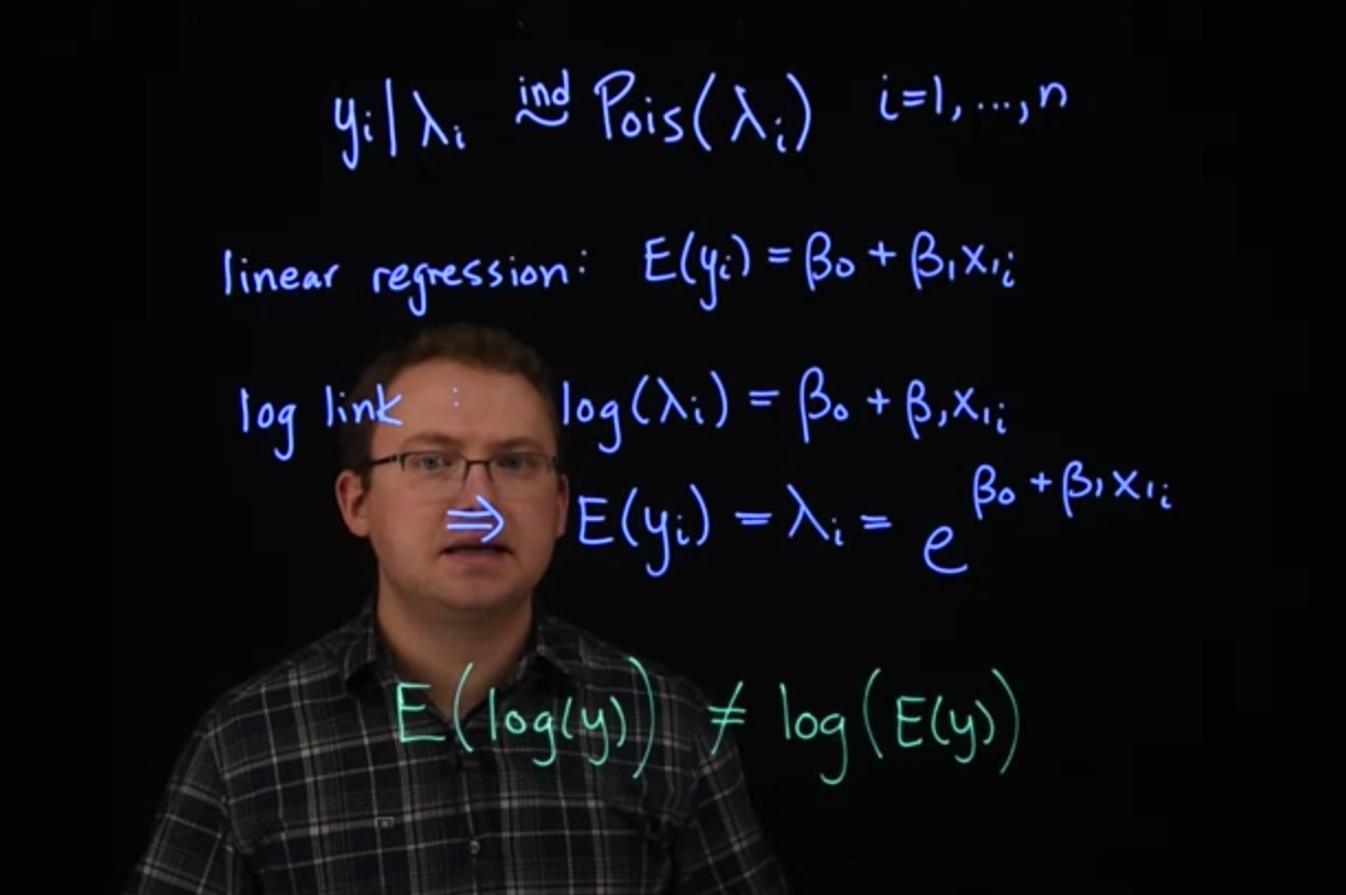
The Poisson distribution provides a natural likelihood for count data.
$$
y_i\mid \lambda+i \stackrel {iid} \sim \mathrm{Pois}(\lambda_i) \qquad i=1, \ldots, n
$$
Here, $\lambda$ conveniently represents the expected value of y $\mathbb{E}[y].$ It turns out that $\lambda$ is also the variance of y $\mathbb{V}ar[y].$ So if we expect a count to be higher, we also expect the variability in counts to go up.
We saw this earlier with the *warp breaks* data.
If we model the mean directly, like we did with linear regression. That is, we had the expected value $y_i$ was directly modeled with this linear form.
$$
\mathbb{E}[y] = \beta_0 + \beta_1x_i \qquad \text{(linear regression)}
$$
We would run into the same problem we did with logistic regression. The expected value has to be greater than zero in the Poisson distribution. To naturally deal with that restriction, we're going to use the logarithmic link function.
So, the log link. That is, that the log of $\lambda_i$ is equal to this linear piece.
log link:
$$
log(\lambda_i) = \beta_0+\beta_1x_i \qquad \text{(log link)}
$$ {#eq-pr-log-link}
$$
\mathbb{E}[y]=\beta_0+\beta_1x_i \qquad \text{(linear regression)}
$$
From this, we can easily recover the expression for the mean itself. That is, we can invert this link function to get the expected value of $y_i,$
$$
\implies \mathbb{E}[y] = \lambda_i = e^{\left(\beta_0+\beta_1x_i \right)}
$$ {#eq-poisson-regression-link}
It might seem like this model is equivalent to fitting a normal linear regression to the log of $y$.
But there are a few key differences.
[In the normal regression, we're modeling the mean of the response directly. So we would be fitting a model to the $\log(y)$. Where we're modeling the expected value of the $\log(y)$. This is different from what we're modeling here, here we're doing the log of the expected value of $y$.]{.mark}
$$
\mathbb{E}[log(y)]\ne log(\mathbb{E}[y])
$$
[These are not equal, they're usually similar, but they're not the same.
Another difference is that we have a separate independent parameter for the variants in a normal regression.
In Poisson regression, the variance is automatically the same as $\lambda$,]{.mark} [which may not always be appropriate]{.mark-red}, as we'll see in an upcoming example.
As usual, we can add more explanatory x variables to the Poisson regression framework.
They can be continuous, categorical, or they could be counts themselves.
If we have three predictor variables $x_i = ( x_{1,i}, x_{2,i}, x_{3,i} ),$ what would the likelihood part of the hierarchical representation of a Poisson regression with logarithmic link look like?
- [ ] $y_i \mid x_i, \beta \overset{\text{ind}}{\sim} \mathrm{Pois} \left( e^{-(\beta_0+\beta_1 x_{1,i}+\beta_2 x_{2,i}+\beta_3 x_{3,i})}\right)$
- [ ] $y_i \mid x_i, \beta \overset{\text{ind}}{\sim} \mathrm{Pois} \left(\beta_0 + \beta_1 x_{1,i} + \beta_2 x_{2,i} + \beta_3 x_{3,i} \right)$
- [x] $y_i \mid x_i, \beta \overset{\text{ind}}{\sim} \mathrm{Pois} \left(e^{\beta_0 + \beta_1 x_{1,i}+\beta_2 x_{2,i}+\beta_3 x_{3,i}}\right)$
- [ ] $y_i \mid x_i, \beta \overset{\text{ind}}{\sim} \mathrm{Pois} \left( \log[ \beta_0 + \beta_1 x_{1,i} + \beta_2 x_{2,i} + \beta_3 x_{3,i} ] \right)$
Here we incorporated the (inverse) link function directly into the likelihood rather than writing it with two lines.
## Poisson regression - JAGS model
\index{dataset!badhealth}
[**doctor visits**]{.column-margin} For an example of Poisson regression, we'll use the `badhealth` data set from the `COUNT` package in `R`.
```{r}
#| label: load-badhealth-data
library("COUNT")
data("badhealth")
#?badhealth
head(badhealth)
```
according to the description:
::: {.callout-note}
## Data Card for `badhealth`
1,127 observations from a 1998 German survey with 3 variables:
1. `numvisit` - number of visits to the doctor in 1998 (**response**)
2. `badh` - $\begin{cases} 1 \qquad \text{ patient claims to be in bad health} \\ 0 \qquad \text{ patient does not claim to be in bad health} \end{cases}$
3. `age` - age of patient
:::
```{r}
#| label: check-missing-data
any(is.na(badhealth))
```
1. remove na
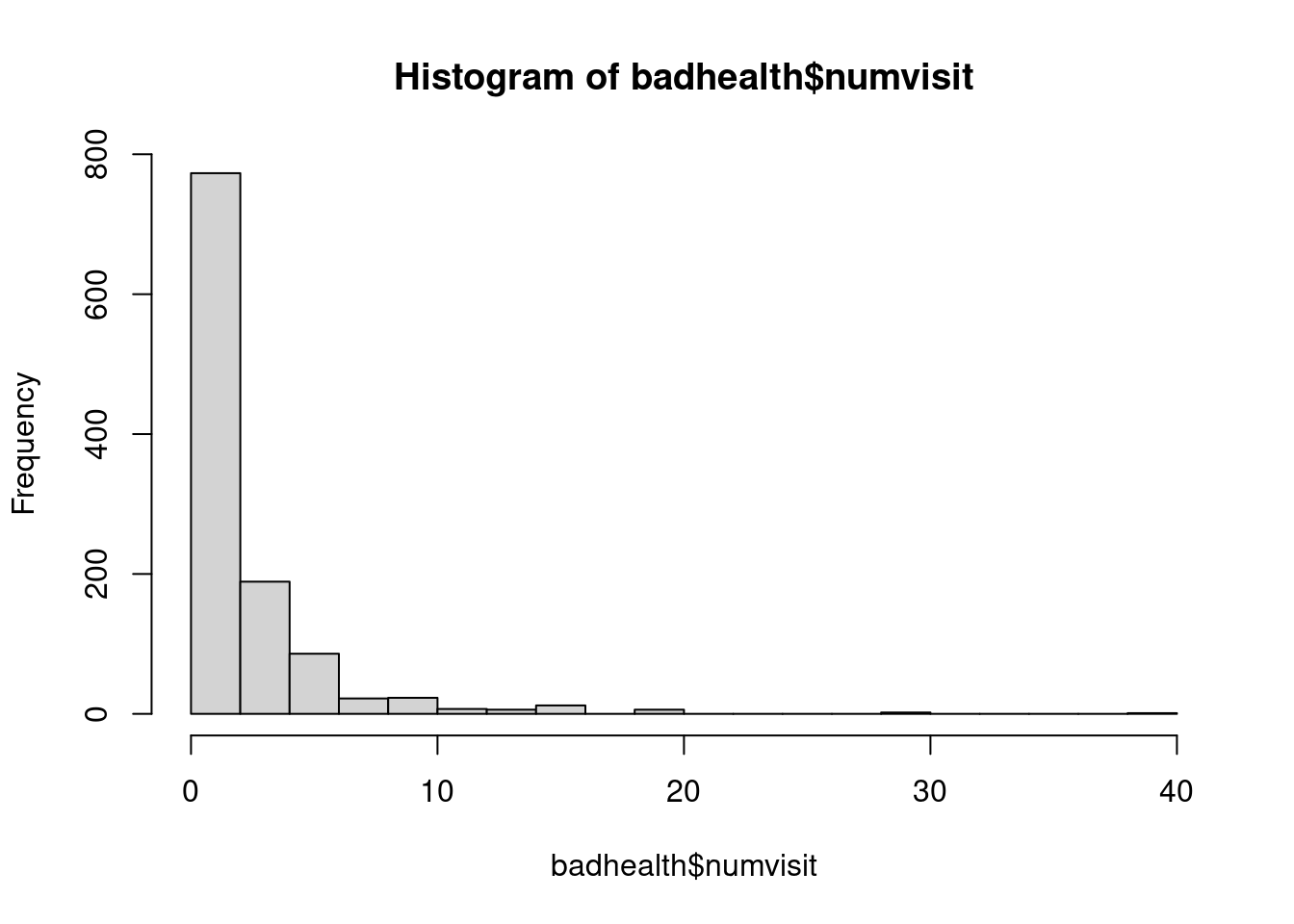
As usual, let's visualize these data.
```{r}
#| label: fig-numvisits-histogram
#| fig-cap: "Histogram of number of doctor visits"
hist(badhealth$numvisit, breaks=20)
```
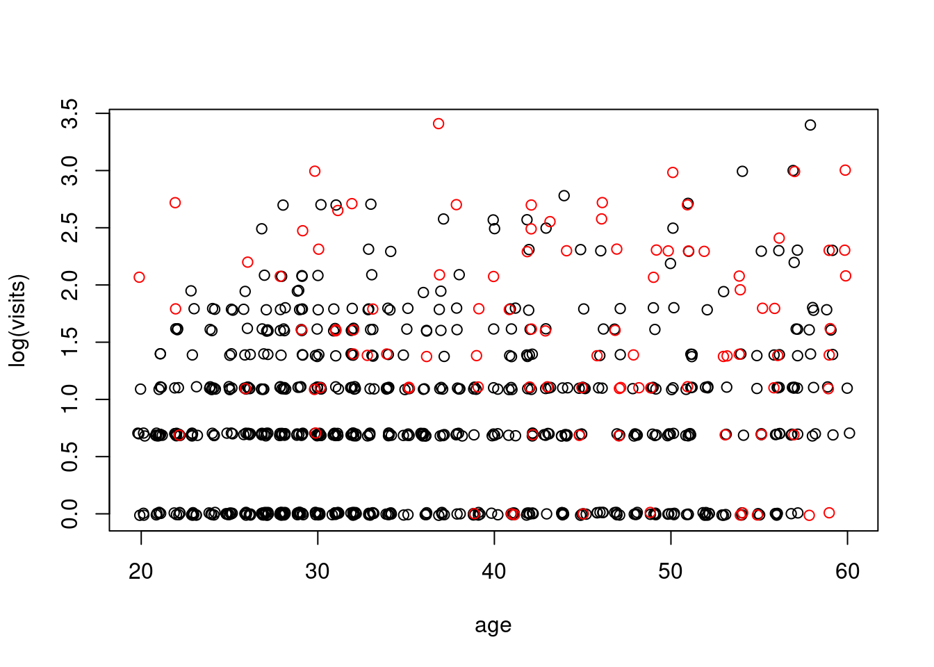
```{r}
#| label: fig-visits-by-age-health
plot(jitter(log(numvisit)) ~ jitter(age), data=badhealth, subset=badh==0, xlab="age", ylab="log(visits)")
points(jitter(log(numvisit)) ~ jitter(age), data=badhealth, subset=badh==1, col="red")
```
### Doctor Visits Model
[**doctor visits**]{.column-margin} It appears that both age and bad health are related to the number of doctor visits. We should include model terms for both variables. [If we believe the age/visits relationship is different between healthy and non-healthy populations, we should also include an interaction term]{.mark}. We will fit the full model here and leave it to you to compare it with the simpler additive model.
```{r}
#| label: load-rjags
library("rjags")
```
```{r}
#| label: define-poisson-jags-model
mod_string = " model {
    for (i in 1:length(numvisit)) {
        numvisit[i] ~ dpois(lam[i])
        log(lam[i]) = int + b_badh*badh[i] + b_age*age[i] + b_intx*age[i]*badh[i]
    }

    int ~ dnorm(0.0, 1.0/1e6)
    b_badh ~ dnorm(0.0, 1.0/1e4)
    b_age ~ dnorm(0.0, 1.0/1e4)
    b_intx ~ dnorm(0.0, 1.0/1e4)
} "

set.seed(102)

data_jags = as.list(badhealth)

params = c("int", "b_badh", "b_age", "b_intx")

mod = jags.model(textConnection(mod_string), data=data_jags, n.chains=3)
update(mod, 1e3)
mod_sim = coda.samples(model=mod, variable.names=params, n.iter=5e3)
mod_csim = as.mcmc(do.call(rbind, mod_sim))
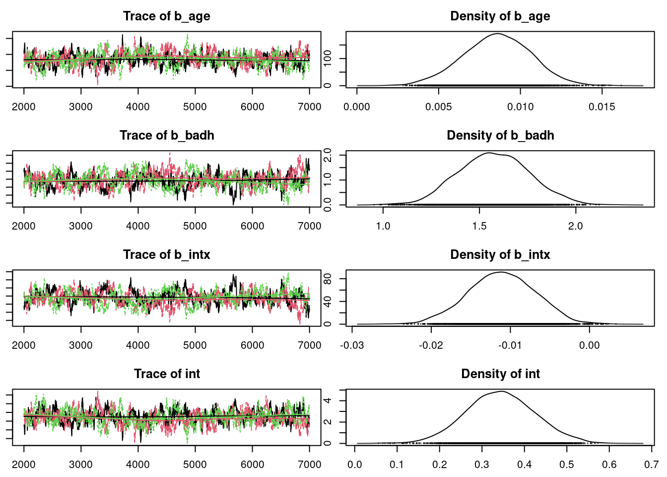
## convergence diagnostics
par(mar = c(2.5, 1, 2.5, 1))
plot(mod_sim)
gelman.diag(mod_sim)
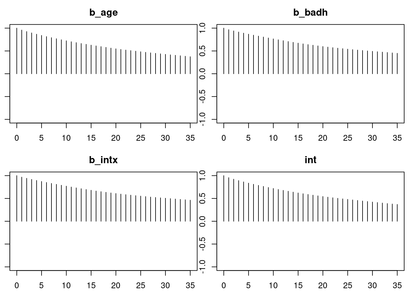
autocorr.diag(mod_sim)
autocorr.plot(mod_csim)
effectiveSize(mod_sim)
## compute DIC
dic = dic.samples(mod, n.iter=1e3)
```
### Model checking - Residuals
> "While inexact models may mislead, attempting to allow for every contingency a priori is impractical. Thus models must be built by an iterative feedback process in which an initial parsimonious model may be modified when diagnostic checks applied to residuals indicate the need." ---G. E. P. Box
To get a general idea of the model's performance, we can look at predicted values and \index{residual analysis} residuals as usual. Don't forget that we must apply the inverse of the link function to get predictions for $\lambda$ .
```{r}
#| label: create-matrix-X
X = as.matrix(badhealth[,-1]) #<1>
X = cbind(X, with(badhealth, badh*age)) #<2>
head(X)
```
1. we drop the first column since it is the column for our `y`.
2. we add a third column with $\mathbb{I}_{badh}\times age$
```{r}
#| label: compute-pmed-coef
(pmed_coef = apply(mod_csim, 2, median)) # <1>
```
1. this are the column medians of the coefficients.
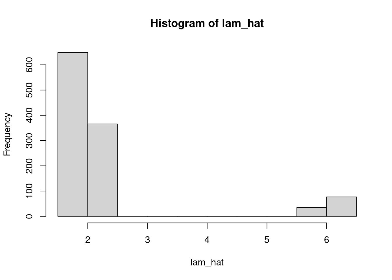
```{r}
#| label: compute-llam-hat
llam_hat = pmed_coef["int"] + X %*% pmed_coef[c("b_badh", "b_age", "b_intx")] # <1>
lam_hat = exp(llam_hat) #<2>
hist(lam_hat)
```
1. $X \cdot \vec b_i$ gives the linear part.
2. $\hat\lambda_i=e^{X \cdot \vec b_i}$ we need to apply the inverse link function
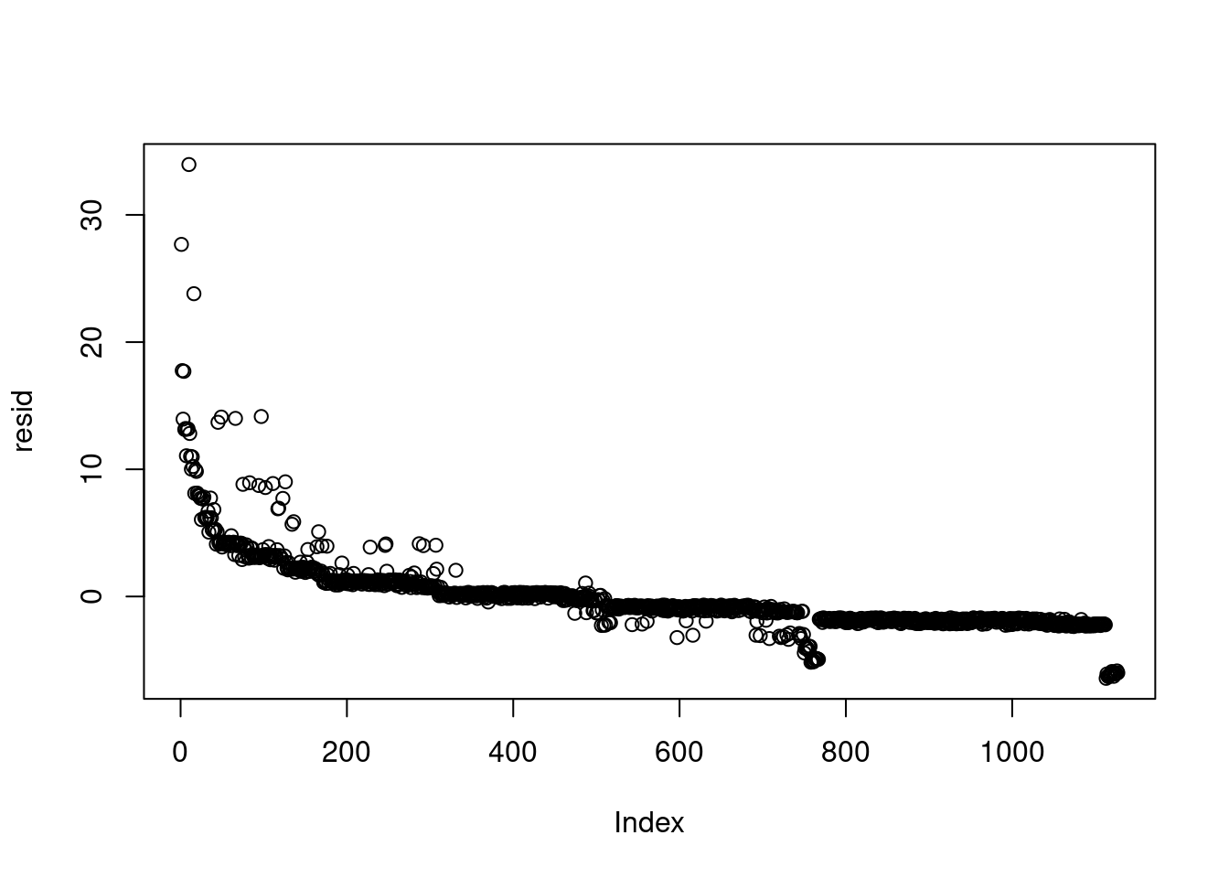
```{r}
#| label: compute-residuals
resid = badhealth$numvisit - lam_hat
plot(resid) # the data were ordered
```
this plot looks bad, it might not be iid but we can ignore the issue since the data is presorted/
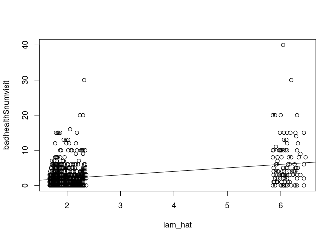
```{r}
#| label: fig-lamhat-vs-numvisit
plot(lam_hat, badhealth$numvisit)
abline(0.0, 1.0)
```
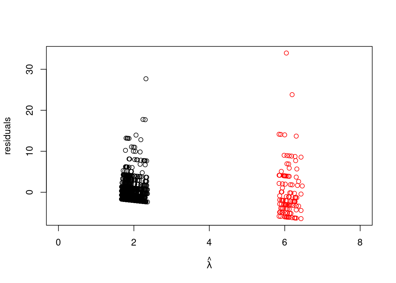
```{r}
#| label: fig-residuals-by-health
plot(lam_hat[which(badhealth$badh==0)], resid[which(badhealth$badh==0)], xlim=c(0, 8), ylab="residuals", xlab=expression(hat(lambda)), ylim=range(resid))
points(lam_hat[which(badhealth$badh==1)], resid[which(badhealth$badh==1)], col="red")
```
It is not surprising that the variability increases for values predicted at higher values since the mean is also the variance in the Poisson distribution. [However, observations predicted to have about two visits should have variance about two, and observations predicted to have about six visits should have variance about six.]{.mark}
```{r}
#| label: compute-variance-resid-healthy
var(resid[which(badhealth$badh==0)])
```
```{r}
#| label: compute-variance-resid-unhealthy
var(resid[which(badhealth$badh==1)])
```
For this data the variance is much bigger this is not the case with these data. This indicates that [either the model fits poorly (meaning the covariates don't explain enough of the variability in the data), or the data are "**overdispersed**" \index{overdispersed} for the Poisson likelihood we have chosen. This is a common issue with count data. If the data are more variable than the Poisson likelihood would suggest, a good alternative is the negative binomial distribution]{#sp-overdispersed .mark}, which we will not pursue here.
## Predictive distributions {#sec-predictive-distributions}
Assuming the model fit is adequate, we can interpret the results.
```{r}
#| label: summarize-mod-sim
summary(mod_sim)
```
[The ***intercept*** is not necessarily *interpretable* here because it corresponds to the number of doctor visits for a healthy 0-year-old. While the number of visits for a newborn baby sounds like interesting information, the youngest person in the data set is 20 years old.]{.mark} In such cases we should avoid making such projections and say that the intercept is an artifact of the model.
- For healthy individuals, it appears that **age** is associated with an *increase* in the Expected *number of doctor visits*.
- **Bad health** is associated with an *increase in expected number of visits*.
- The interaction coefficient is interpreted as an adjustment to the age coefficient for people in bad health. Hence, for people with bad health, age is essentially unassociated with number of visits.
### Predictive distributions
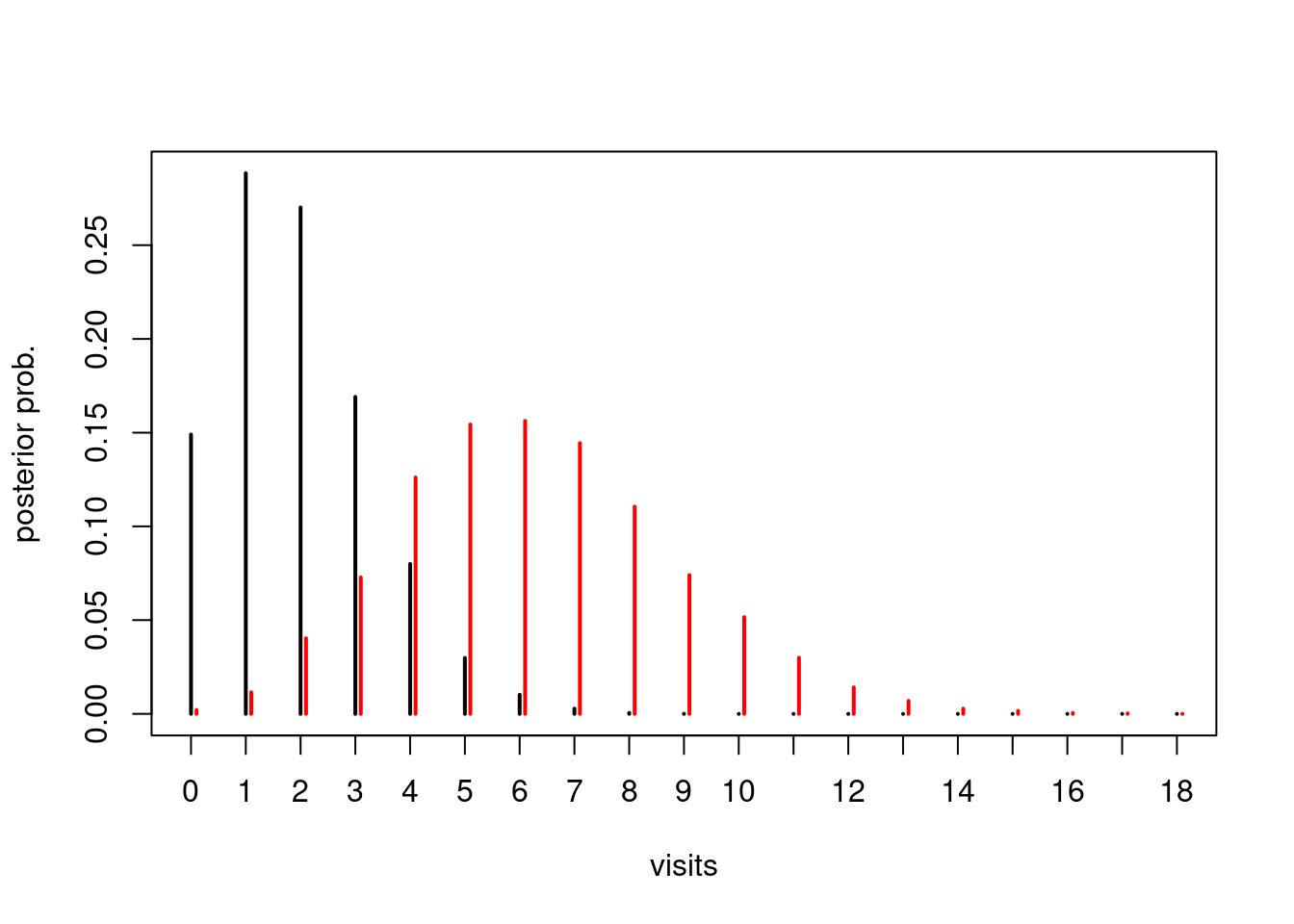
Let's say we have two people aged 35, one in good health and the other in poor health. [**Q. What is the posterior probability that the individual with poor health will have more doctor visits?**]{.column-margin}
[This goes beyond the posterior probabilities we have calculated comparing expected responses in previous lessons. Here we will create Monte Carlo samples for the **responses themselves**. This is done by taking the Monte Carlo samples of the model parameters, and for each of those, drawing a sample from the likelihood]{.mark}.
Let's walk through this.
First, we need the $x$ values for each individual. We'll say the healthy one is Person 1 and the unhealthy one is Person 2. Their $x$ values are:
```{r}
#| label: define-x-values
x1 = c(0, 35, 0) # <1>
x2 = c(1, 35, 35) # <2>
```
1. good health person's data (bad_health_indicator=0,age=35,age\*indicator=0)
2. bad health person's (bad_health_indicator=1,age=35,age\*indicator=35)
The posterior samples of the model parameters are stored in `mod_csim`:
```{r}
#| label: show-mod-csim-head
head(mod_csim)
```
First, we'll compute the linear part of the predictor:
```{r}
#| label: compute-log-lambda
loglam1 = mod_csim[,"int"] + mod_csim[,c(2,1,3)] %*% x1
loglam2 = mod_csim[,"int"] + mod_csim[,c(2,1,3)] %*% x2
```
Next we'll apply the inverse link:
```{r}
#| label: compute-lambda
lam1 = exp(loglam1)
lam2 = exp(loglam2)
```
The final step is to use these samples for the $\lambda$ parameter for each individual and simulate actual number of doctor visits using the likelihood:
```{r}
#| label: compute-nsim
(n_sim = length(lam1))
```
we have distribution of 15000 samples of $\lambda$ for each person.
```{r}
#| label: compute-y1-y2
y1 = rpois(n=n_sim, lambda=lam1) #<1>
y2 = rpois(n=n_sim, lambda=lam2) #<1>
plot(table(factor(y1, levels=0:18))/n_sim, pch=2, ylab="posterior prob.", xlab="visits")
points(table(y2+0.1)/n_sim, col="red")
```
```{r}
#| label: fig-posterior-predictive
plot(table(factor(y1, levels=0:18))/n_sim, pch=2, ylab="posterior prob.", xlab="visits")
points(table(y2+0.1)/n_sim, col="red")
```
Finally, we can answer the original question: What is the probability that the person with poor health will have more doctor visits than the person with good health?
```{r}
#| label: compute-prob-y2-greater-y1
mean(y2 > y1)
```
Because we used our posterior samples for the model parameters in our simulation (the `loglam1` and `loglam2` step above), this posterior predictive distribution on the number of visits for these two new individuals naturally account for our uncertainty in the model estimates. This is a more honest/realistic distribution than we would get if we had fixed the model parameters at their MLE or posterior means and simulated data for the new individuals.
## Prior sensitivity analysis {#sec-prior-sensitivity-analysis}
\index{prior sensitivity analysis}
\index{modeling decisions}
\index{sensitivity analysis}
[**Q. How do you justify the model you choose?**]{.column-margin} When communicating results from any analysis, a responsible statistician will report and justify *modeling decisions*, especially assumptions. In a Bayesian analysis, there is an additional assumption that is open to scrutiny: the *choices of prior distributions*. In the models considered so far in this course, there are an infinite number of prior distributions we could have chosen from.
When communicating results from any analysis, a responsible statistician will report and justify *modeling decisions*, especially assumptions. In a Bayesian analysis, there is another assumption that is open to scrutiny: the *choices of prior distributions*. In the models considered so far in this course, there are an infinite number of prior distributions we could have chosen from.
[**Q. How do you justify the priors you choose?**]{.column-margin} If they truly represent your beliefs about the parameters before analysis and the model is appropriate, then the posterior distribution truly represents your updated beliefs. If you don't have any strong beliefs beforehand, there are often default, reference, or non-informative prior options, and you will have to select one. However, a collaborator or a boss (indeed, somebody somewhere) may not agree with your choice of prior. [One way to increase the credibility of your results is to repeat the analysis under a variety of priors, and report how the results differ as a result.]{.mark} This process is called *prior sensitivity analysis*.
[At a minimum you should always report your choice of model and prior]{.mark}. If you include a sensitivity analysis, select one or more alternative priors and describe how the results of the analysis change. If they are sensitive to the choice of prior, you will likely have to explain both sets of results, or at least explain why you favor one prior over another. [If the results are not sensitive to the choice of prior, this is evidence that the data are strongly driving the results. It suggests that different investigators coming from different backgrounds should come to the same conclusions.]{.mark}
[If the purpose of your analysis is to establish a hypothesis, it is often prudent to include a "skeptical" prior which does not favor the hypothesis.]{.mark} Then, if the posterior distribution still favors the hypothesis despite the unfavorable prior, you will be able to say that the data substantially favor the hypothesis. This is the approach we will take in the following example, continued from the previous lesson.
### Poisson regression example
[**doctor visits**]{.column-margin} Let's return to the example of number of doctor visits. We concluded from our previous analysis of these data that both bad health and increased age are associated with more visits. Suppose the burden of proof that bad health is actually associated with more visits rests with us, and we need to convince a skeptic.
First, let's re-run the original analysis and remind ourselves of the posterior distribution for the `badh` (bad health) indicator.
```{r}
#| label: load-libraries-sensitivity
library("COUNT")
library("rjags")

data("badhealth")
```
```{r}
#| label: define-model-string
mod_string = " model {
    for (i in 1:length(numvisit)) {
        numvisit[i] ~ dpois(lam[i])
        log(lam[i]) = int + b_badh*badh[i] + b_age*age[i] + b_intx*age[i]*badh[i]
    }

    int ~ dnorm(0.0, 1.0/1e6)
    b_badh ~ dnorm(0.0, 1.0/1e4)
    b_age ~ dnorm(0.0, 1.0/1e4)
    b_intx ~ dnorm(0.0, 1.0/1e4)
} "

set.seed(102)

data_jags = as.list(badhealth)

params = c("int", "b_badh", "b_age", "b_intx")

mod = jags.model(textConnection(mod_string), data=data_jags, n.chains=3)
update(mod, 1e3)

mod_sim = coda.samples(model=mod,
                        variable.names=params,
                        n.iter=5e3)
mod_csim = as.mcmc(do.call(rbind, mod_sim))
```
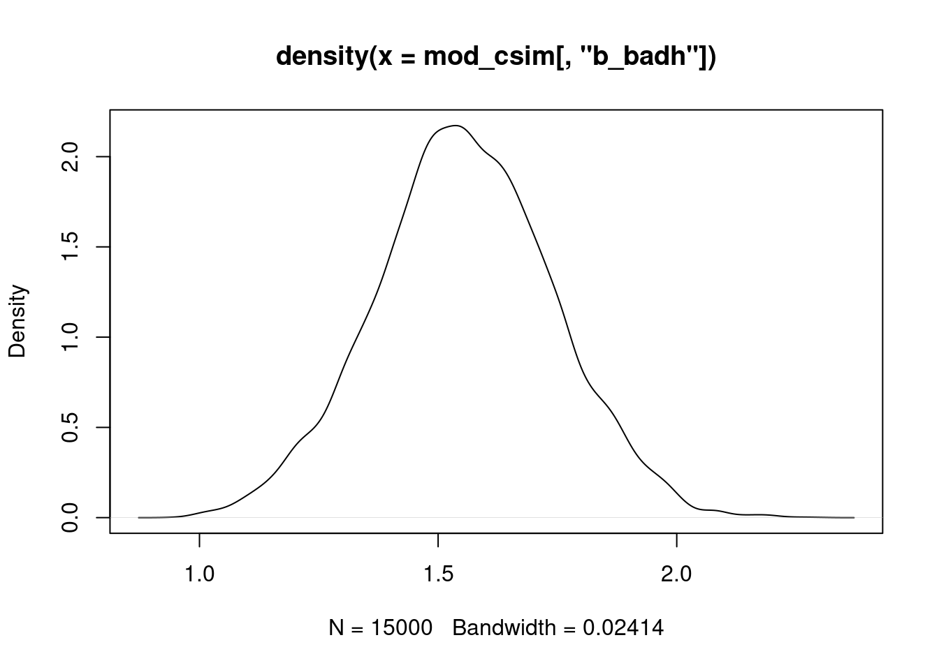
```{r}
#| label: fig-density-bbadh
plot(density(mod_csim[,"b_badh"]))
```
Essentially all of the posterior probability mass is above 0, suggesting that this coefficient is positive (and consequently that bad health is associated with more visits). We obtained this result using a relatively noninformative prior. What if we use a prior that strongly favors values near 0? Let's repeat the analysis with a normal prior on the `badh` coefficient that has mean 0 and standard deviation 0.2, so that the prior probability that the coefficient is less than 0.6 is $>0.998$ . We'll also use a small variance on the prior for the interaction term involving `badh` (standard deviation 0.01 because this coefficient is on a much smaller scale).
```{r}
#| label: define-model2-string
mod2_string = " model {
    for (i in 1:length(numvisit)) {
        numvisit[i] ~ dpois(lam[i])
        log(lam[i]) = int + b_badh*badh[i] + b_age*age[i] + b_intx*age[i]*badh[i]
    }

    int ~ dnorm(0.0, 1.0/1e6)
    b_badh ~ dnorm(0.0, 1.0/0.2^2)
    b_age ~ dnorm(0.0, 1.0/1e4)
    b_intx ~ dnorm(0.0, 1.0/0.01^2)
} "

mod2 = jags.model(textConnection(mod2_string), data=data_jags, n.chains=3)
update(mod2, 1e3)

mod2_sim = coda.samples(model=mod2,
                        variable.names=params,
                        n.iter=5e3)
mod2_csim = as.mcmc(do.call(rbind, mod2_sim))
```
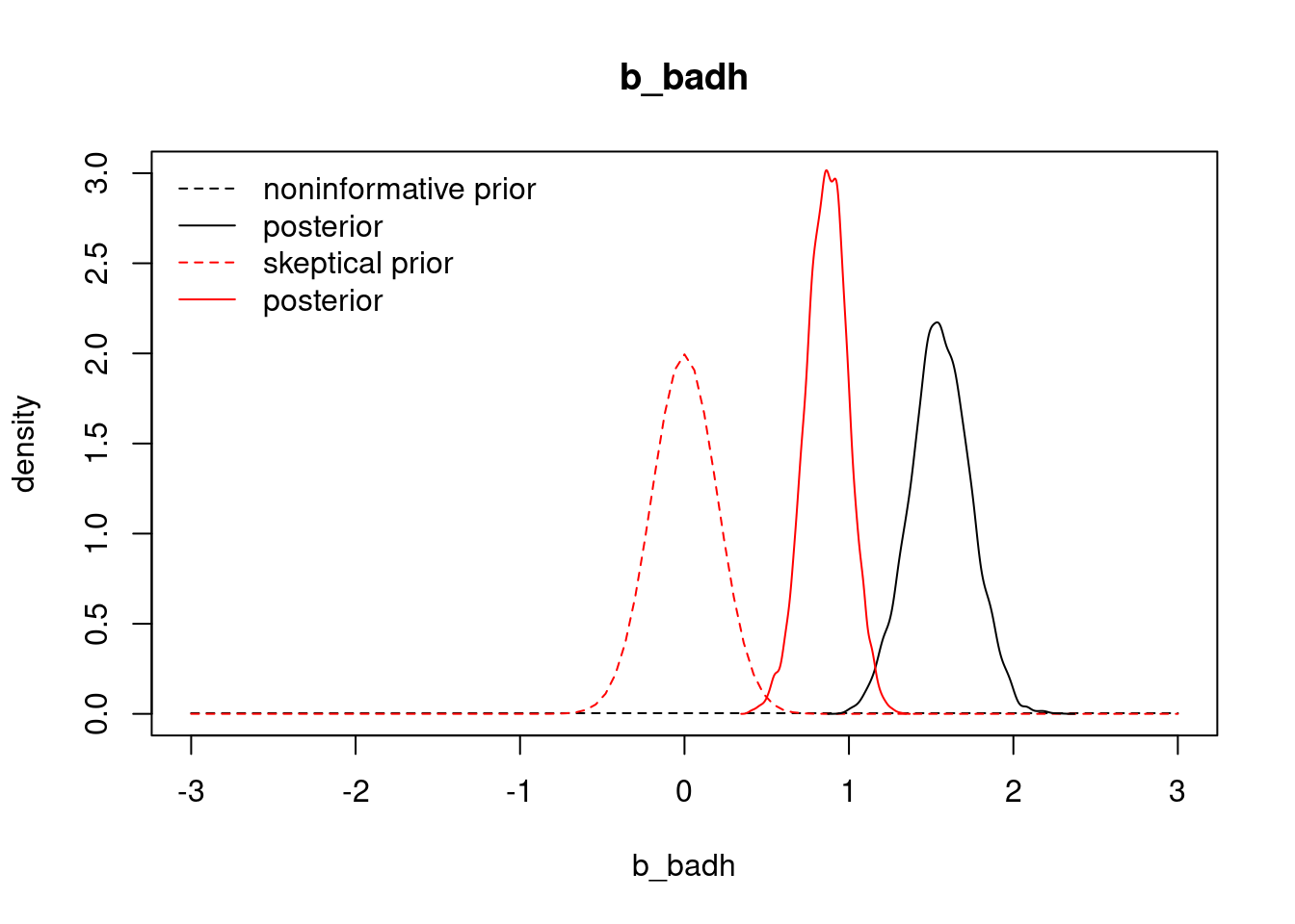
How did the posterior distribution for the coefficient of `badh` change?
```{r}
#| label: fig-prior-and-posterior-comparison
curve(dnorm(x, mean=0.0, sd=sqrt(1e4)), from=-3.0, to=3.0, ylim=c(0.0, 3.0), lty=2,
      main="b_badh", ylab="density", xlab="b_badh")
curve(dnorm(x, mean=0.0, sd=0.2), from=-3.0, to=3.0, col="red", lty=2, add=TRUE)
lines(density(mod_csim[,"b_badh"]))
lines(density(mod2_csim[,"b_badh"]), col="red")
legend("topleft", legend=c("noninformative prior", "posterior", "skeptical prior", "posterior"),
       lty=c(2,1,2,1), col=rep(c("black", "red"), each=2), bty="n")
```
Under the skeptical prior, our posterior distribution for `b_badh` has significantly dropped to between about 0.6 and 1.1. Although the strong prior influenced our inference on the magnitude of the bad health effect on visits, it did not change the fact that the coefficient is significantly above 0. In other words: even under the skeptical prior, bad health is associated with more visits, with posterior probability near 1.
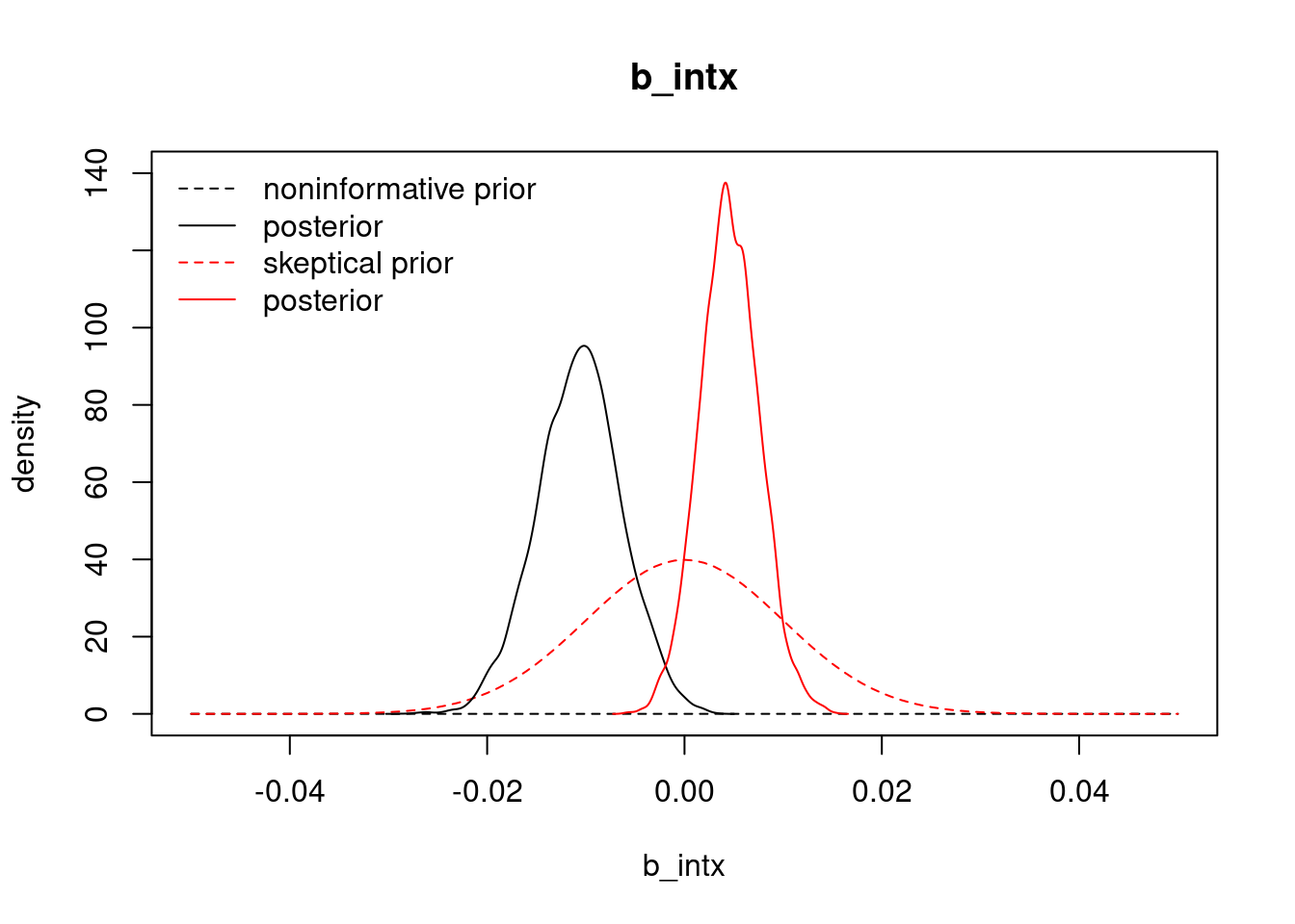
We should also check the effect of our skeptical prior on the interaction term involving both age and health.
```{r}
#| label: fig-prior-and-posterior-comparison-intx
curve(dnorm(x, mean=0.0, sd=sqrt(1e4)), from=-0.05, to=0.05, ylim=c(0.0, 140.0), lty=2,
      main="b_intx", ylab="density", xlab="b_intx")
curve(dnorm(x, mean=0.0, sd=0.01), from=-0.05, to=0.05, col="red", lty=2, add=TRUE)
lines(density(mod_csim[,"b_intx"]))
lines(density(mod2_csim[,"b_intx"]), col="red")
legend("topleft", legend=c("noninformative prior", "posterior", "skeptical prior", "posterior"),
       lty=c(2,1,2,1), col=rep(c("black", "red"), each=2), bty="n")
```
```{r}
#| label: compute-mean-bintx-positive
mean(mod2_csim[,"b_intx"] > 0) # posterior probability that b_intx is positive
```
The result here is interesting. Our estimate for the interaction coefficient has gone from negative under the non-informative prior to positive under the skeptical prior, so the result is sensitive. In this case, because the skeptical prior shrinks away much of the bad health main effect, it is likely that this interaction effect attempts to restore some of the positive effect of bad health on visits. Thus, despite some observed prior sensitivity, our conclusion that bad health positively associates with more visits remains unchanged.
## Overdispersed model
Recall that the **Negative Binomial** can be used to model overdispersed count data.
`stan` has three parameterizations for the **Negative Binomial**.
The first looks like similar to a binomial parameterization:
$$
\text{NegBinomial}(y~|~\alpha,\beta) = \binom{y +
\alpha - 1}{\alpha - 1} \, \left( \frac{\beta}{\beta+1}
\right)^{\!\alpha} \, \left( \frac{1}{\beta + 1} \right)^{\!y} \!.
$$
$$
\mathbb{E}[y] = \frac{\alpha}{\beta} \ \ \text{ and } \ \ \text{Var}[Y] = \frac{\alpha}{\beta^2} (\beta + 1).
$$
we can sample from this using the following statement
``` r
n ~ neg_binomial(alpha, beta)
```
But this parameterization if not a match to the Poisson model, so we move on
The second parametrization $\mu \in \mathbb{R}^+$ and $\phi \in \mathbb{R}^+$:
$$
\mathrm{NegBinomial2}(n \mid \mu, \phi) = \binom{n + \phi - 1}{n} \,
\left( \frac{\mu}{\mu+\phi} \right)^{\!n} \, \left(
\frac{\phi}{\mu+\phi} \right)^{\!\phi}
$$
$$
\mathbb{E}[n] = \mu \ \ \text{ and } \ \ \ \mathbb{V}\text{ar}[n] = \mu + \frac{\mu^2}{\phi}
$$
we can sample from this using the following statement
``` r
n ~ neg_binomial_2(mu, phi)
```
And there is a third parametrization
$$
NegBinomial2Log(y\mid\mu,\phi) = NegBinomial2(y\mid exp(\eta),\phi).
$$
we can sample from this using the following statement:
``` r
y \~ **neg_binomial_2\_log**(y\|mu, phi)`
```
`jags` has just one parameterization:
$$
f(y \mid r, p) = \frac{\Gamma(y+r)}{\Gamma(r)\Gamma(y+1)}p^r(1-p)^y
$$
We think of the Negative Binomial Distribution as the probability of completing $y$ successful trials allowing for $r$ failures in a sequence of $(y+r)$ Bernoulli trials where success is defined as drawing (with replacement) a white ball from an urn of white and black balls with a probability `p` of success.
$$
\mathbb{E}[Y] = \mu = { r(1-p) \over p } \qquad \text{ and } \qquad \mathbb{V}\text{ar}[Y] = \mu + \frac{\mu^2}{r}
$$
### Transformations:
Since we want to have a model corresponding to a poisson regression we will transform the model as follows:
If we set $p = {\text{r} \over {r} + \lambda }$ then the mean becomes : $\lambda$
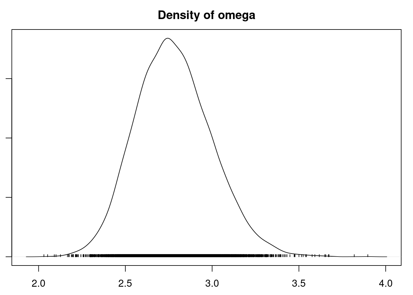
and if we also set $r= {\lambda^2 \over \omega}$ then the variance becomes a sum of $\lambda + \omega$ where $\omega$ is our **over dispersion** term.
$$
\omega = \lambda^2 / r
$$
$$
\begin{aligned}
\mathbb{E}[Y] &= { r(1-p) \over p }
\\ &= rp^{-1} -r
\\ & \stackrel {sub\ p} = {\cancel{r}(\bcancel{r}+\lambda) \over \cancel{r}} - \bcancel{r}
\\ &= \lambda \mathbb{V}\text{ar}[Y]
\\ &= { (1-p) r \over p^2 }
\\ & \stackrel {sub \ \lambda } = {1 \over p} \lambda
\\ & \stackrel {sub p} = \lambda { (r+ \lambda) \over r}
\\ &= {\lambda r + \lambda^2 \over r }
\\ &= 1 \lambda + {\lambda^2 \over r}
\\ &\stackrel { sub \ \omega}= \lambda + \omega
\end{aligned}
$$
Where we interpret $\lambda$ as the mean and $\omega$ as the overdispersion \index{overdispersion}
```{r}
#| label: load-libraries-overdispersed
library("rjags")
library("COUNT")
data("badhealth")
```
```{r}
#| label: define-overdispersed-model
mod3_string = "
model {
for (i in 1:length(numvisit)) {
mu[i] = b0 + b_badh*badh[i] + b_age*age[i] + b_intx*age[i]*badh[i] # <1>
lambda[i] = exp(mu[i]) # <2>
p[i] = r / (r + lambda[i]) # <3>
numvisit[i] ~ dnegbin(p[i], r) # <4>
resid[i] = numvisit[i] - p[i] # <5>
}
## Priors
b0 ~ dnorm(0.0, 1.0/1e6) # <6>
b_badh ~ dnorm(0.0, 1.0/0.2^2) # <7>
b_age ~ dnorm(0.0, 1.0/1e4) # <8>
b_intx ~ dnorm(0.0, 1.0/0.01^2) # <9>
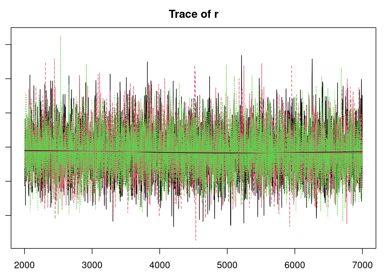
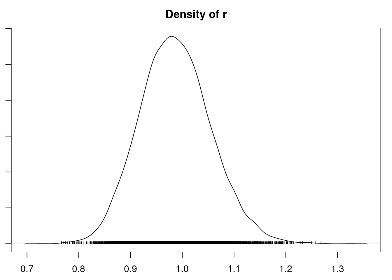
r ~ dunif(0,50) # <10>
## extra deterministic parameters
omega <- pow(mean(lambda),2)/2
#theta <- pow(1/mean(p),2) # <11>
#scale <- mean((1-p)/p) # <12>
}"
data3_jags = as.list(badhealth)
mod3 = jags.model(textConnection(mod3_string), data=data3_jags, n.chains=3)
update(mod3, 1e3) # <13>
params3 = c("b_intx", "b_badh", "b_age", 'over_disp', 'b0','omega','r')
mod3_sim = coda.samples(model=mod3, variable.names=params3, n.iter=5e3) # <14>
mod3_csim = as.mcmc(do.call(rbind, mod3_sim)) # <15>
(dic3 = dic.samples(mod3, n.iter=1e3)) # <16>
```
1. the linear part
2. lambda corresponds to the parameter used in the Poisson regression
3. p is the success parameter
4. we draw from the negative binomial distribution
5. sampling using the parametrization of the Negative Binomial distribution.
6. normal prior for intercept `b0`
7. normal prior for `b_badh`
8. normal prior for `b_age`
9. normal prior for `b_intx`
10. uniform prior for `over_disp` - at the upper limit of 50 **NegBin** converges to **Poisson** see [@jackman2009 p. 280]
11. theta param
12. scale param
13. burn in
14. sample
15. stack samples from the chains
16. estimate the DIC
```{r}
#| label: gelman-diag-mod3-sim
gelman.diag(mod3_sim )
```
```{r}
#| label: raftery-diag-mod3-sim
raftery.diag(mod3_sim)
```
```{r}
#| label: autocorr-diag-mod3-sim
autocorr.diag(mod3_sim)
```
```{r}
#| label: effectiveSize-mod3-sim
effectiveSize(mod3_sim)
```
```{r}
#| label: summary-mod3-sim
summary(mod3_sim)
```
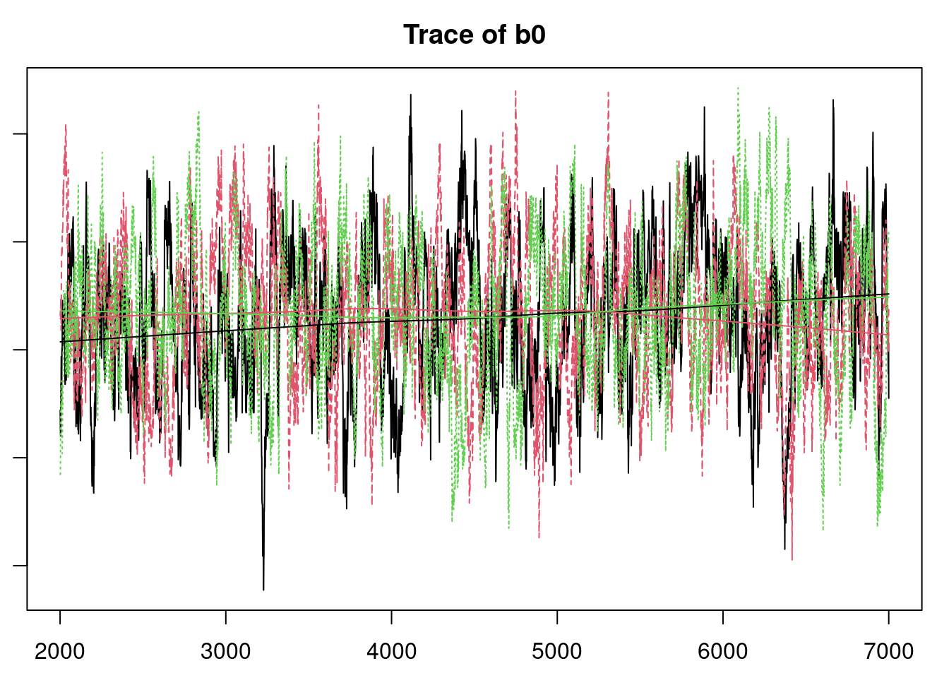
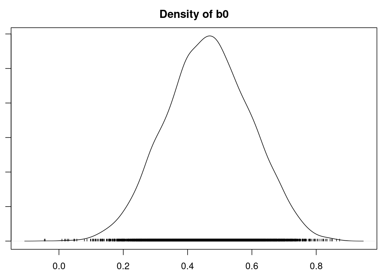
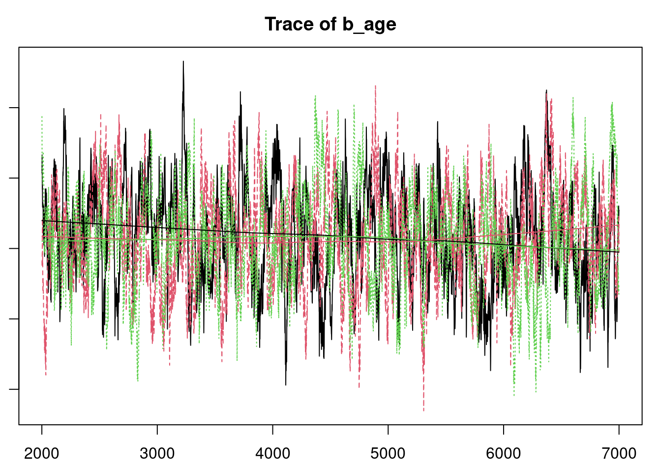
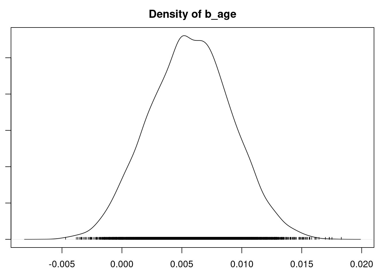
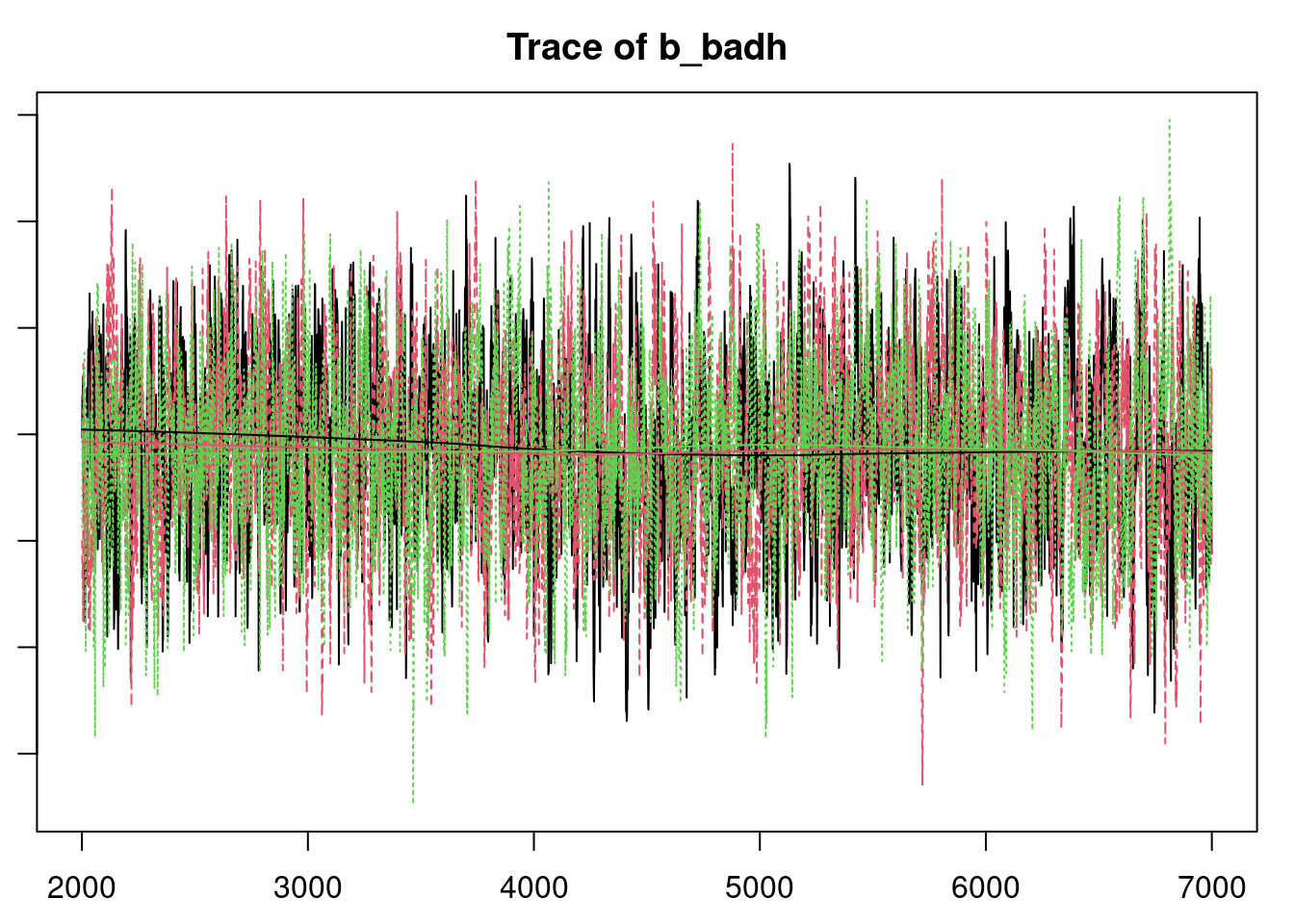
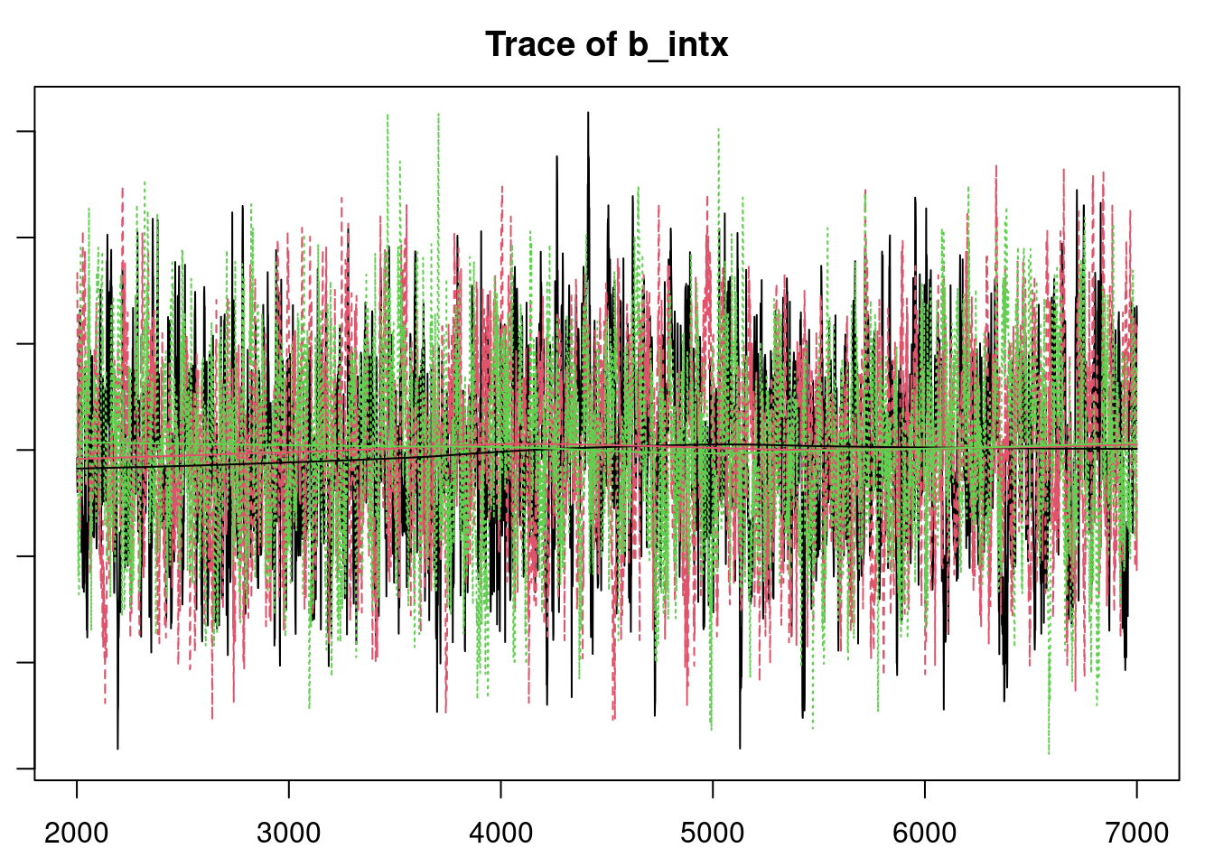
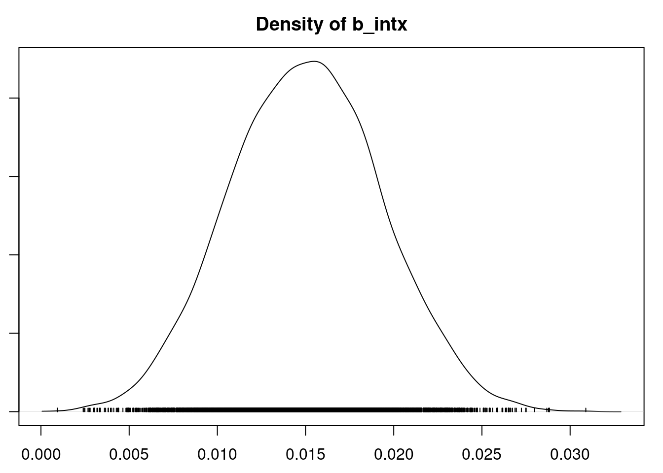
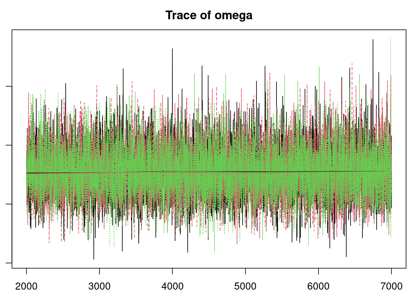
```{r}
#| label: fig-overdisperesed-convergence
#| layout-ncol: 2
par(mar = c(2.5, 1, 2.5, 1))
plot(mod3_sim, auto.layout = FALSE)
```
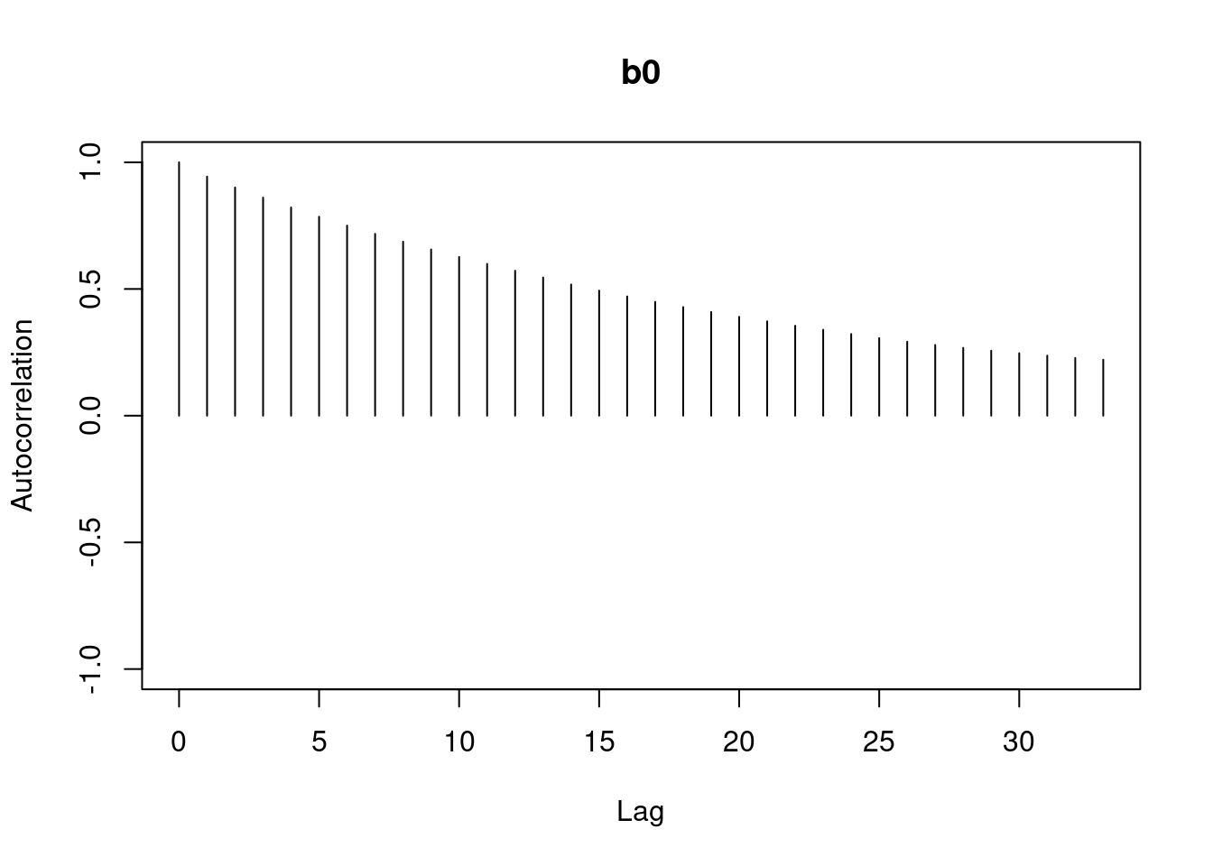
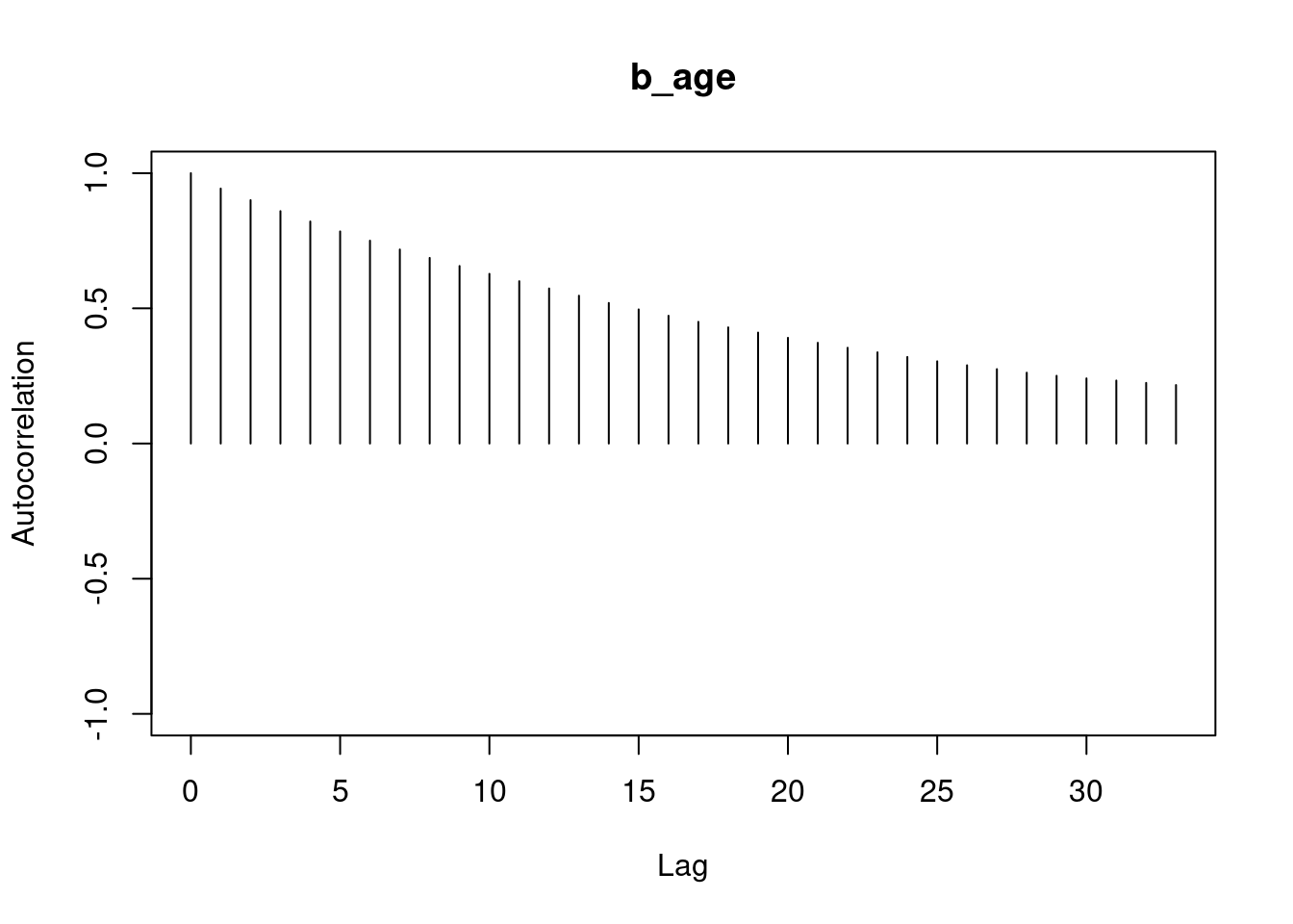
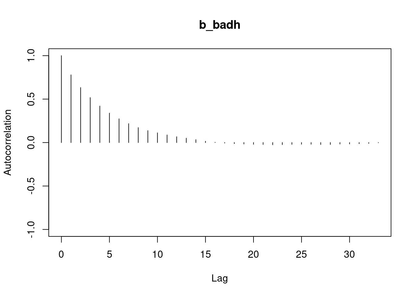
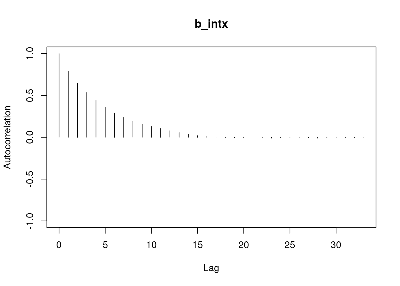
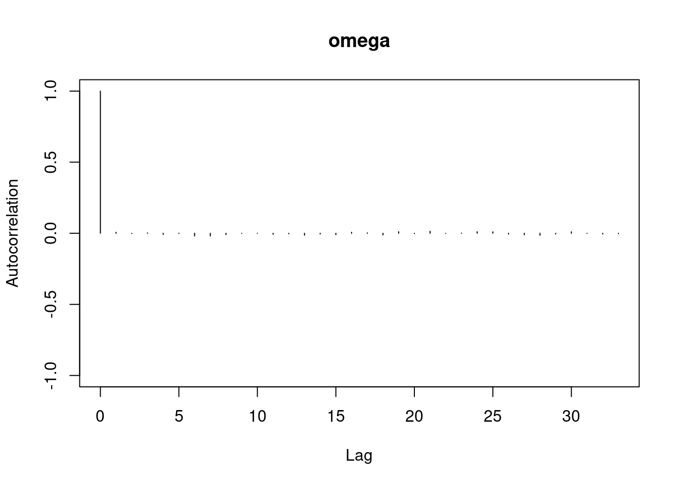
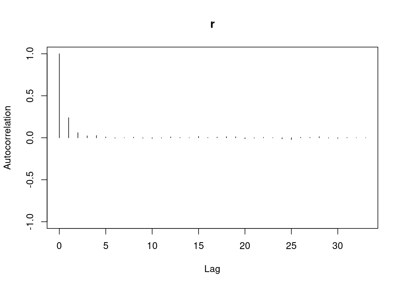
```{r}
#| label: fig-autocorr-plot-mod3-csim
#| layout-ncol: 1
autocorr.plot(mod3_csim,auto.layout = FALSE)
```
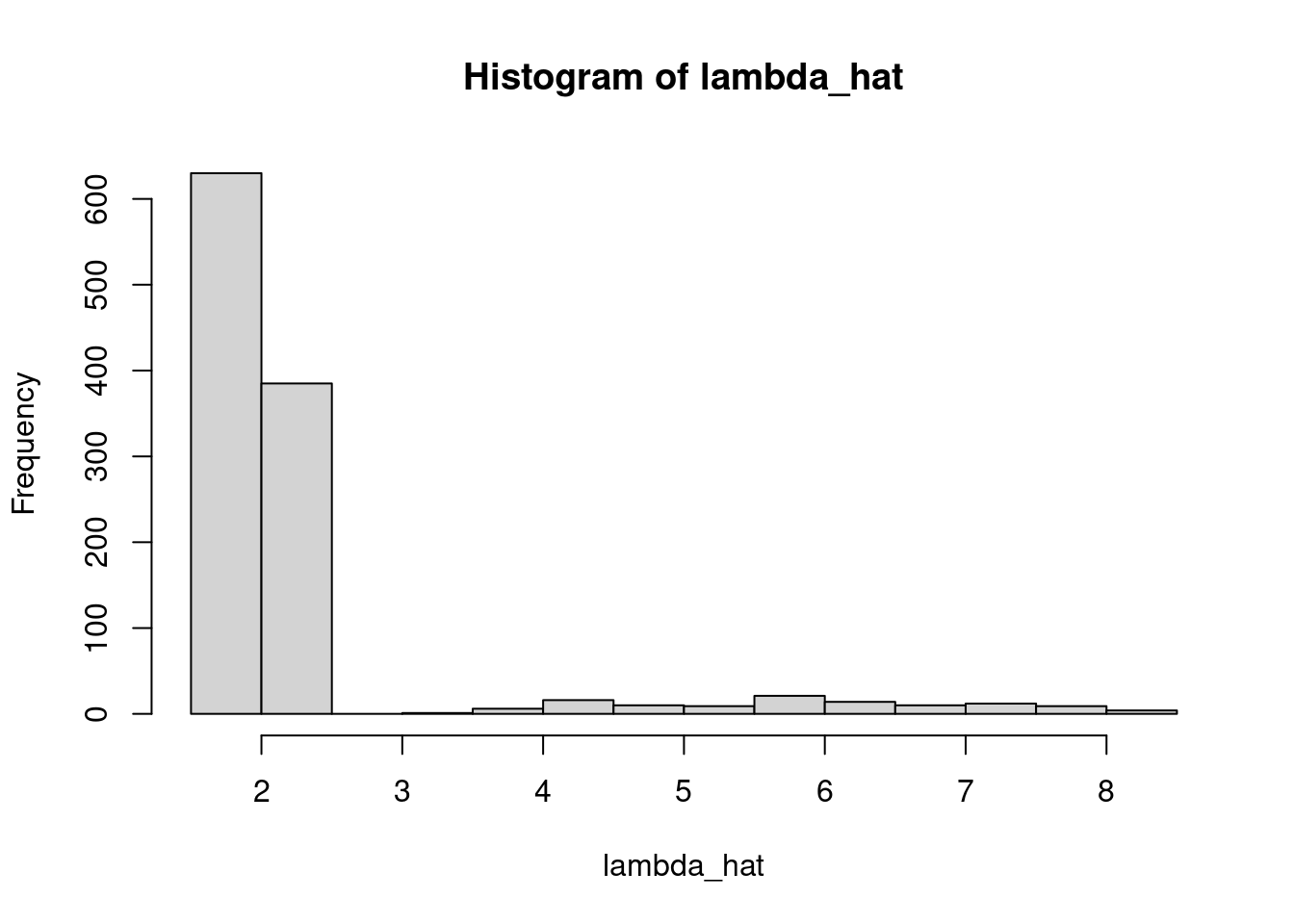
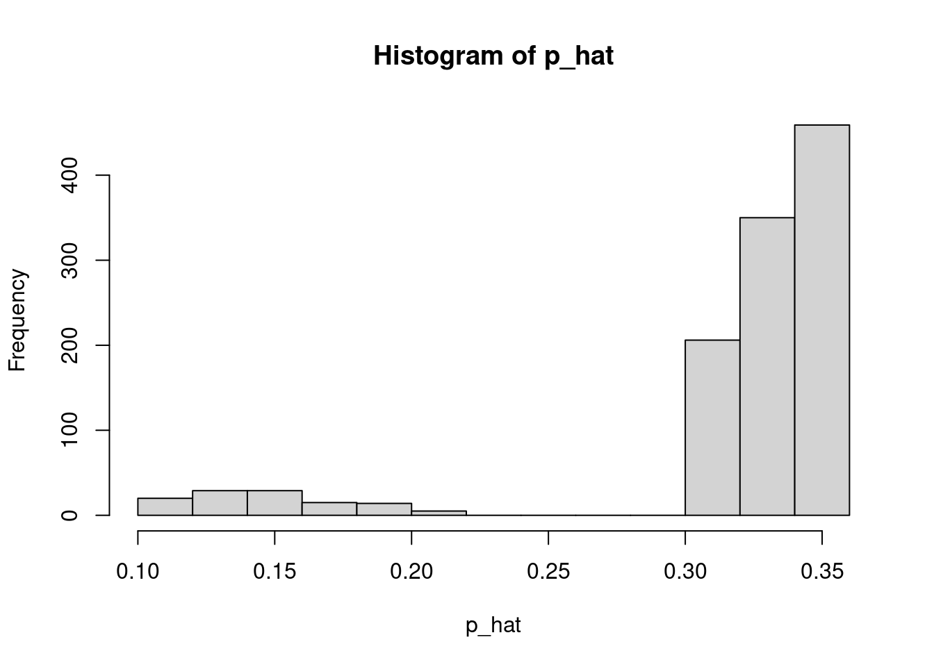
```{r}
#| label: compute-X-pmed-r
X = as.matrix(badhealth[,-1])
X = cbind(X, with(badhealth, badh*age))
(pmed_coef = apply(mod3_csim, 2, median))
(r = pmed_coef["r"] )
mu_hat = pmed_coef["b0"] + X %*% pmed_coef[c("b_badh", "b_age", "b_intx")]
lambda_hat = exp(mu_hat)
p_hat = r / (r + lambda_hat)
hist(lambda_hat)
hist(p_hat)
```
residuals
```{r}
#| label: compute-resid-p_hat
resid = badhealth$numvisit - p_hat
head(resid)
```
```{r}
#| label: fig-residuals-plot
#| fig-cap: "Plot of residuals"
plot(resid) # the data were ordered
```
```{r}
#| label: tbl-head-mod3_csim
#| tbl-cap: "First few rows of mod3_csim"
head(mod3_csim)
```
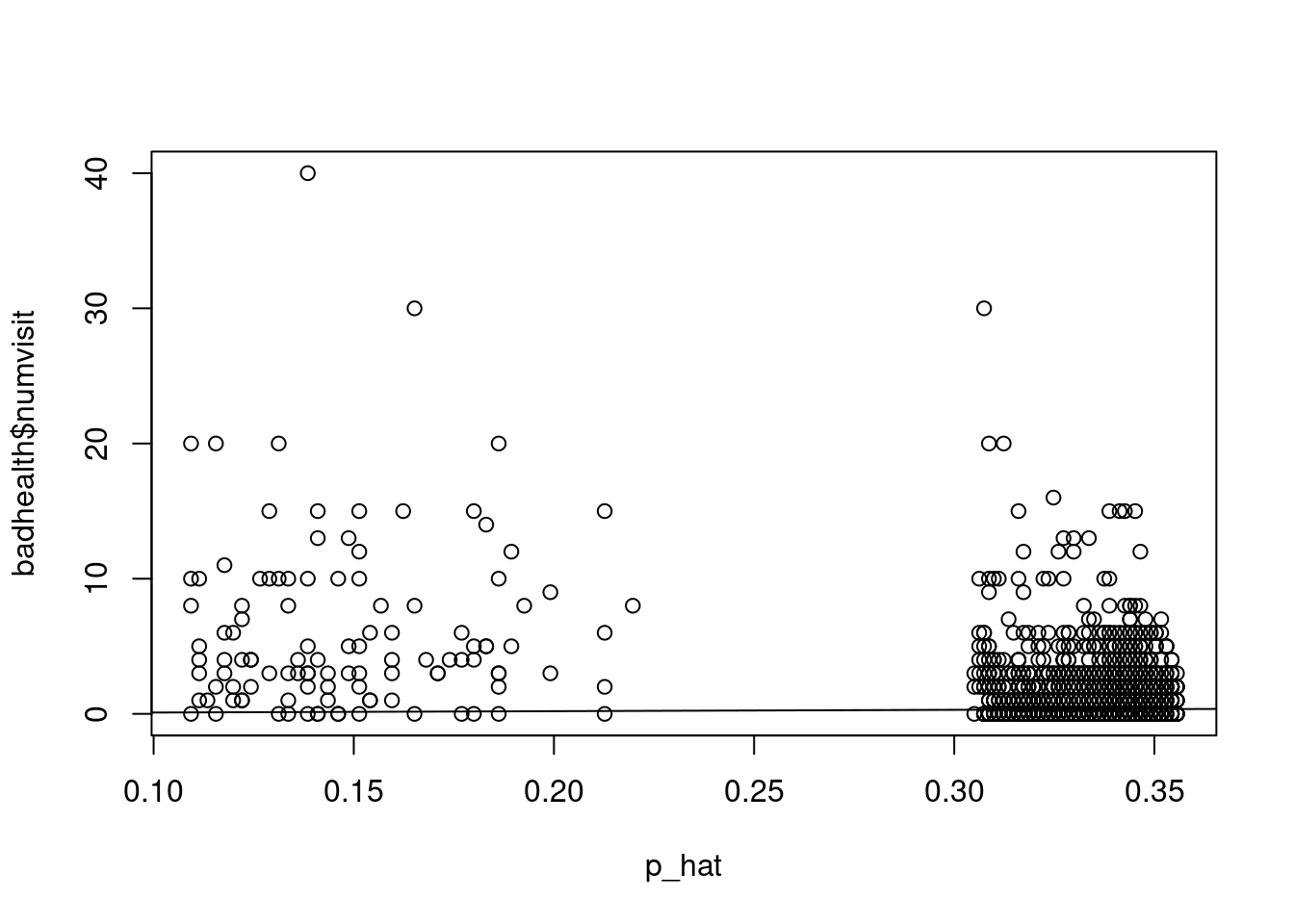
```{r}
#| label: fig-p_hat-vs-numvisit
#| fig-cap: "Plot of p_hat vs numvisit"
plot(p_hat, badhealth$numvisit)
abline(0.0, 1.0)
```
```{r}
#| label: fig-p_hat-vs-resid
#| fig-cap: "Plot of p_hat vs residuals, colored by health status"
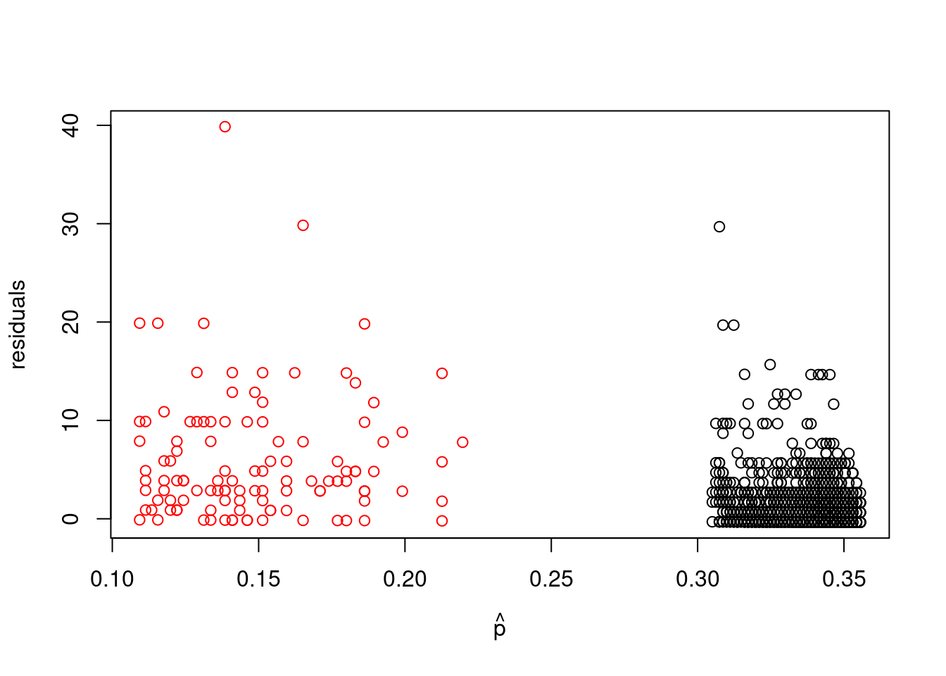
plot(p_hat[which(badhealth$badh==0)], resid[which(badhealth$badh==0)], xlim=range(p_hat), ylab="residuals", xlab=expression(hat(p)), ylim=range(resid))
points(p_hat[which(badhealth$badh==1)], resid[which(badhealth$badh==1)], col="red")
```
```{r}
#| label: compute-variance-resid-by-health
var(resid[which(badhealth$badh==0)])
var(resid[which(badhealth$badh==1)])
```