## simulate data


set.seed(1)
AR.model = list(order = c(2, 0, 0), ar = c(0.5,0.4))
y.sample = arima.sim(n=100,model=AR.model,sd=0.1)


plot(y.sample,type='l',xlab='time',ylab='')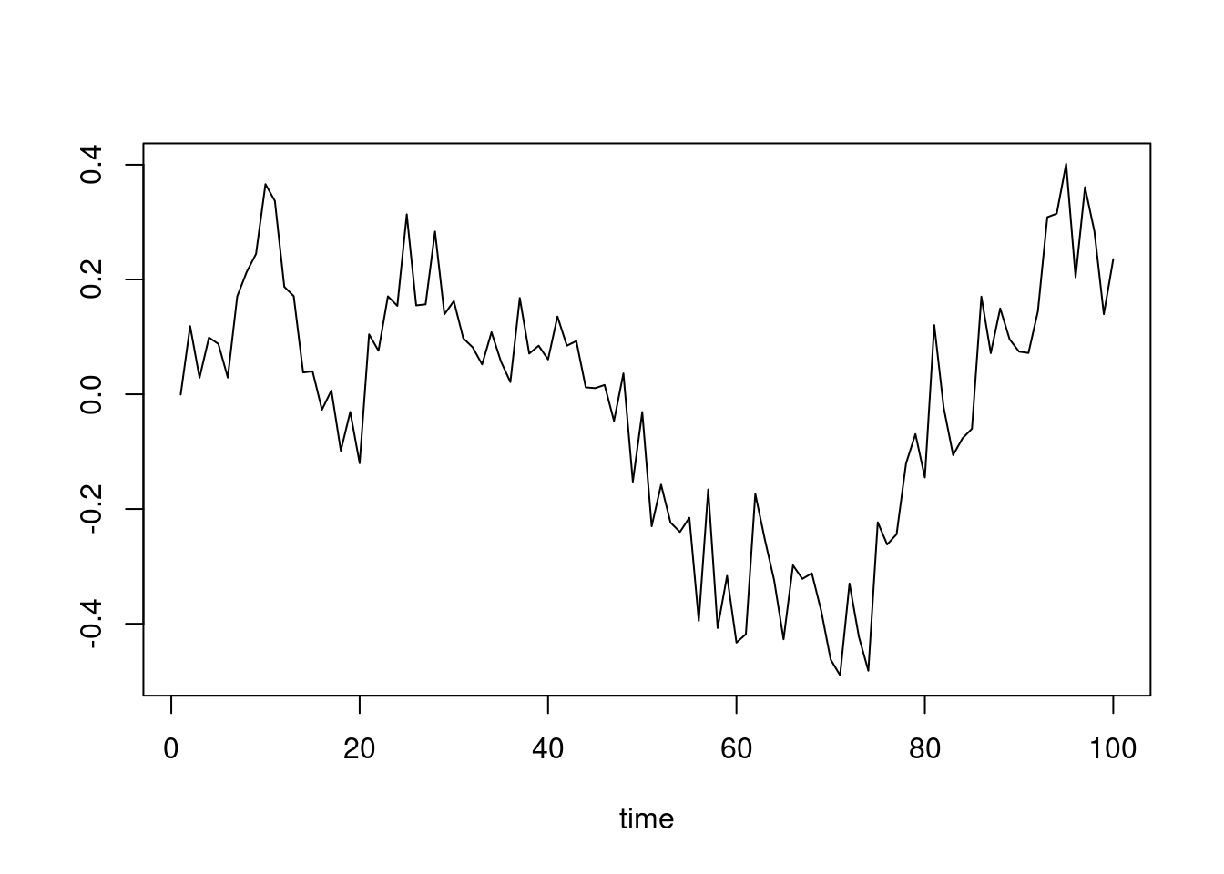
Time Series
Note: we have already covered Akaike information criteria (AIC) and Bayesian information criteria (BIC) a few times in this specialization. In Section 81.1 we discussed how to use BIC to select the number of components in a mixture model. In Section 107.1 we will see how to use AIC and BIC to select the order of an AR process. In Section 95.3 we discussed how to use BIC to select the order of an AR process.
To fit an AR(p) model to real data we need to determine the order p of the AR process.
One approach is to treat this as a model selection problem , where we want to select the model with the best fit from multiple candidate models with different orders p.
One possible way is to repeat the analysis for different values of model order p and choose the best model based on some criteria. The two most widely known criteria are the so-called Akaike information criteria, AIC and the Bayesian Information criteria, BIC.
Note: I have pointed out before that while we can approach estimating the the number of component of a Mixture or the order of an AR(p) process as a hyperparameter tuning problem which involves training multiple models and using model selection criteria to pick the best one. Seems intuitive but is this the best way to do it?
Another approach might be to incorporate the number of components or the order of the AR process as a random variable in our model, and then use Bayesian inference to estimate its posterior distribution. This way we can avoid the need for model selection criteria and instead directly estimate the uncertainty around the number of components or the order of the AR process. I think this is also more or less how this is handled in bayesian switching models, where the number of different phases (stats) in the time series is treated as a random variable and the model is trained to infer the number of phases and their characteristics. C.f. (Davidson-Pilon 2015, chap. 2) where this is called switch point detection or change point analysis
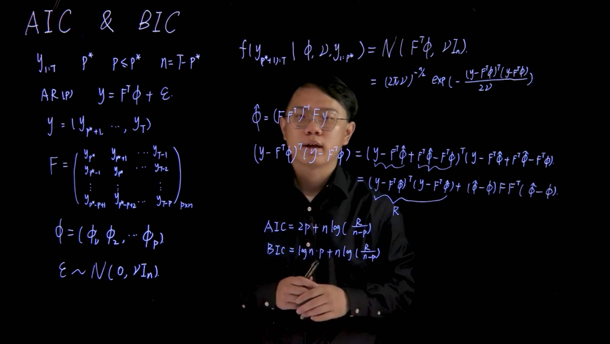
Recall that our model in Equation 104.4 is:
\mathbf{y}\sim \mathcal{N}(\mathbf{F}^\top \boldsymbol{\phi},\nu\mathbf{I}_n),\quad \boldsymbol{\phi}\sim \mathcal{N}(\mathbf{m}_0,\nu\mathbf{C}_0),\quad \nu\sim IG(\frac{n_0}{2},\frac{d_0}{2}) \tag{101.4}
We now describe how to select the order of AR process using AIC or BIC.
We simulate an AR process of order 2, and implement the AIC and BIC criteria to check if the best model selected has order 2.
Firstly, the following code simulate an AR(2) process with 100 observations. The process is simulated from
y_t=0.5y_{t−1}+0.4y_{t−2}+\varepsilon_t,\qquad \varepsilon_t\sim\mathcal{N}(0,0.12)
## simulate data
set.seed(1)
AR.model = list(order = c(2, 0, 0), ar = c(0.5,0.4))
y.sample = arima.sim(n=100,model=AR.model,sd=0.1)
plot(y.sample,type='l',xlab='time',ylab='')
The ACF and PACF plot of the simulated data is shown below.
par(mfrow=c(1,2))


acf(y.sample,main="",xlab='Lag')


pacf(y.sample,main="",xlab='Lag')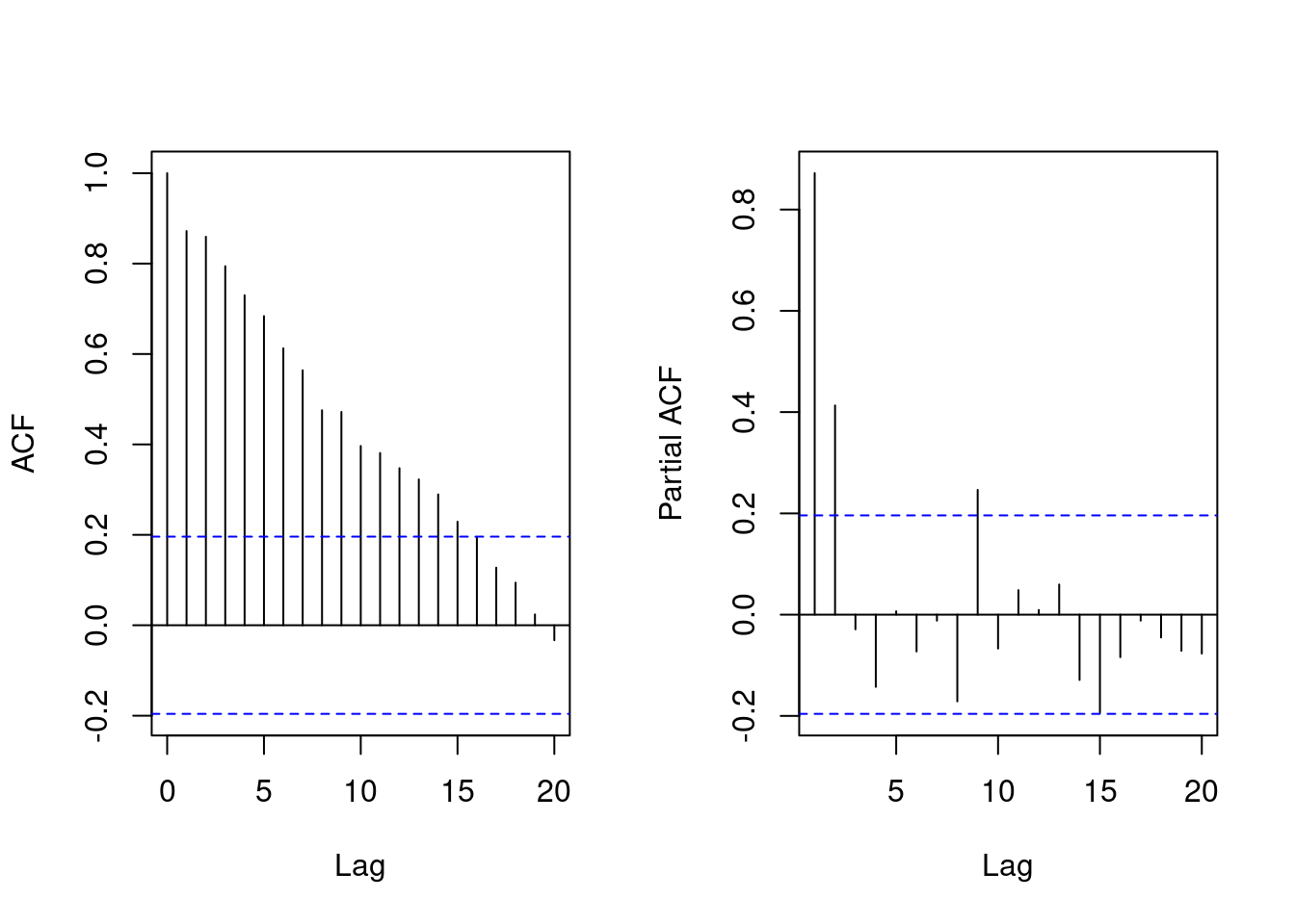
For our case, we fix p^∗=15 as the maximum order of the AR process. The AIC and BIC are calculated for different values of p where 1≤p≤p^∗=15.
T=100
we will use the latter 85 observations for the analysis. We plot both AIC and BIC for different values of p where 1≤p≤p^∗=15 as follows:
n.all=length(y.sample)
p.star=15
Y=matrix(y.sample[(p.star+1):n.all],ncol=1)
sample.all=matrix(y.sample,ncol=1)
n=length(Y)
p=seq(1,p.star,by=1)

design.mtx=function(p_cur){
  Fmtx=matrix(0,ncol=n,nrow=p_cur)
  for (i in 1:p_cur) {
    start.y=p.star+1-i
    end.y=start.y+n-1
    Fmtx[i,]=sample.all[start.y:end.y,1]
  }
  return(Fmtx)
}

criteria.ar=function(p_cur){
  Fmtx=design.mtx(p_cur)
  beta.hat=chol2inv(chol(Fmtx%*%t(Fmtx)))%*%Fmtx%*%Y
  R=t(Y-t(Fmtx)%*%beta.hat)%*%(Y-t(Fmtx)%*%beta.hat)
  sp.square=R/(n-p_cur)
  aic=2*p_cur+n*log(sp.square)
  bic=log(n)*p_cur+n*log(sp.square)
  result=c(aic,bic)
  return(result)
}

criteria=sapply(p,criteria.ar)

plot(p,criteria[1,],type='p',pch='a',col='red',xlab='AR order p',ylab='Criterion',main='',
    ylim=c(min(criteria)-10,max(criteria)+10))
points(p,criteria[2,],pch='b',col='blue')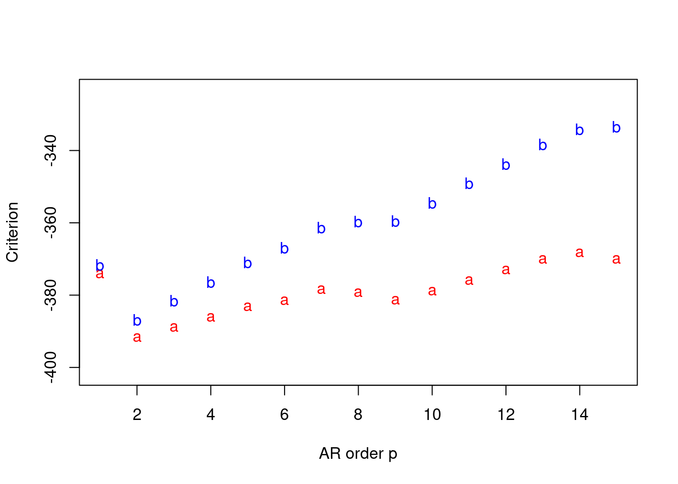
Since for AIC and BIC criteria, we both prefer model with smallest criterion, from the plot we will use p=2 which is the same as the order we used to simulate the data.
DIC is a somewhat Bayesian version of AIC. We will use DIC later to determine the number of mixture component after introducing the mixture AR model for time series.
Suppose we have some data y and we assume y is generated from some distribution, as follows:
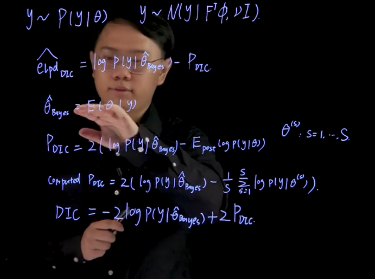
y\sim \mathbb{P}r(y\mid \theta) \qquad y \sim \mathcal{N}(F^\top \boldsymbol{\phi},\nu\mathbf{I}),
The general formula for calculating DIC arises from the modal estimation of expected log density, defined as \widehat{elpd}_{DIC}
expected loss density function (elpd) which is given by: \widehat{elpd}_{DIC} = log(p(y\mid \hat{\theta}_{Bayes}))- P_{DIC}
where \hat{\theta}_{Bayes} is the posterior mean of \theta given y, defined as:
\hat{\theta}_{Bayes} = \mathbb{E}[\theta \mid y]
and P_{DIC} is the effective number of parameters, which is defined as: P_{DIC} = 2 \log(Pr(y\mid \hat{\theta}_{Bayes})) - \mathbb{E}_{post} \log(Pr(y \mid \hat{\theta}))
This expectation is an average of \theta taken over the posterior distribution. This posterior distribution does not in general have a closed form solution. However, we can approximate it using Monte Carlo sampling, i.e. we can use posterior samples \hat{\theta}^{(s)} to approximate the expectation as follows:
\text{For samples } \theta^{(s)}: S=1...s
\text{Computed } P_{DIC} = 2 \log(\mathbb{P}r(y\mid \hat{\theta}_{Bayes})) - \frac{1}{S}\sum_{s=1}^{S} \log(\mathbb{P}r(y\mid \hat{\theta}^{(s)}))
DIC = -2\log(\mathbb{P}r(y\mid \hat{\theta}_{Bayes})) + 2P_{DIC}
DIC is a modal comparison criteria, its value may not be very useful by itself. But later on when we also compute the assay for serum mixture models, we can compare the DIC value for every model and select the best model by choosing the model with the smallest DIC.
We use the same simulated data as an example to illustrate how we can compute DIC in R. That is, we simulate 100 observations from
y_t=0.5y_{t-1}+0.4y_{t-2}+\epsilon_t,\quad \epsilon_t\sim N(0,0.1^2)
## simulate data


set.seed(1)
AR.model = list(order = c(2, 0, 0), ar = c(0.5,0.4))
y.sample = arima.sim(n=100,model=AR.model,sd=0.1)


plot(y.sample,type='l',xlab='time',ylab='')
Posterior Inference From previous analysis, we already know we should fit an AR(2) model to the data. Using the Bayesian conjugate analysis of AR model learned from the first module, we fit AR(2) model with prior m_0 = (0, 0)^T, \quad C_0 = I_2, \quad n_0 = 2, \quad d_0 = 2
We obtain 5000 posterior samples and plot their empirical distribution as follows.
library(mvtnorm)


n.all=length(y.sample)
p=2
m0=matrix(rep(0,p),ncol=1)
C0=diag(p)
n0=2
d0=2

Y=matrix(y.sample[3:n.all],ncol=1)
Fmtx=matrix(c(y.sample[2:(n.all-1)],y.sample[1:(n.all-2)]),nrow=p,byrow=TRUE)
n=length(Y)

e=Y-t(Fmtx)%*%m0
Q=t(Fmtx)%*%C0%*%Fmtx+diag(n)
Q.inv=chol2inv(chol(Q))
A=C0%*%Fmtx%*%Q.inv
m=m0+A%*%e
C=C0-A%*%Q%*%t(A)
n.star=n+n0
d.star=t(Y-t(Fmtx)%*%m0)%*%Q.inv%*%(Y-t(Fmtx)%*%m0)+d0

n.sample=5000


nu.sample=rep(0,n.sample)
phi.sample=matrix(0,nrow=n.sample,ncol=p)


for (i in 1:n.sample) {
  set.seed(i)
  nu.new=1/rgamma(1,shape=n.star/2,rate=d.star/2)
  nu.sample[i]=nu.new
  phi.new=rmvnorm(1,mean=m,sigma=nu.new*C)
  phi.sample[i,]=phi.new
}


par(mfrow=c(1,3))
hist(phi.sample[,1],freq=FALSE,xlab=expression(phi[1]),main="")
lines(density(phi.sample[,1]),type='l',col='red')
hist(phi.sample[,2],freq=FALSE,xlab=expression(phi[2]),main="")
lines(density(phi.sample[,2]),type='l',col='red')
hist(nu.sample,freq=FALSE,xlab=expression(nu),main="")
lines(density(nu.sample),type='l',col='red')
Now using the formula for DIC, we first need to compute \log p(y\mid \hat{\theta}_{Bayes}) . In our example, this is
\sum_{t=p+1}^{T} \log(N(y_t \mid f_t^T \phi_{Bayes}, \nu_{Bayes})) {#sec-capstone-dic-log-py}
which can be computed as follows:
cal_log_likelihood=function(phi,nu){
  mu.y=t(Fmtx)%*%phi
  log.lik=sapply(1:length(mu.y), function(k){dnorm(Y[k,1],mu.y[k],sqrt(nu),log=TRUE)})
  sum(log.lik)
}


phi.bayes=colMeans(phi.sample)
nu.bayes=mean(nu.sample)


log.lik.bayes=cal_log_likelihood(phi.bayes,nu.bayes)
cat("log.lik.bayes=",log.lik.bayes,"\n")
log.lik.bayes= 62.34778 Then, to calculate p_{DIC}, we need to calculate
\frac{1}{S}\sum_{s=1}^{S}\log p(y\mid \hat{\theta}^{(s)})
which in our case is
\frac{1}{S}\sum_{s=1}^{S}\sum_{t=p+1}^{T}\log(N(y_t\mid f_t^T\phi^{(s)},\nu^{(s)}))
It can be calculated by the following code:
post.log.lik=sapply(1:5000, function(k){cal_log_likelihood(phi.sample[k,],nu.sample[k])})
E.post.log.lik=mean(post.log.lik)


p_DIC=2*(log.lik.bayes-E.post.log.lik)
cat("p_DIC=",p_DIC,"\n")
p_DIC= 0.8483731 Now, using the formula for DIC, we can finally compute it. The value of DIC may not make sense now. It will be useful later when we compute DIC for mixture models and select the best model among them.
DIC=-2*log.lik.bayes+2*p_DIC
cat("DIC=",DIC,"\n")
DIC= -122.9988