---
date: 2024-11-04
title: "The AR($p$) process"
subtitle: Time Series Analysis
description: "The AR($p$) process, its state-space representation, the characteristic polynomial, and the forecast function"
categories:
- Bayesian Statistics
- Time Series
keywords:
- Autoregressive Models
- time series
- stability
- order of an AR process
- characteristic lag polynomial
- autocorrelation function
- ACF
- partial autocorrelation function
- PACF
- smoothing
- State Space Model
- ARMA process
- ARIMA
- moving average
- AR($p$) process
- R code
- notes
- Coursera
---
::: {.callout-note}
## Learning Objectives
- [x] Define an **AR($p$)**, or [autoregressive process of order p]{.mark} and use **R** to obtain samples from such process
- [x] Define ARIMA (autoregressive moving average) models (honors)
- [x] Perform posterior inference for the AR($p$) under the conditional likelihood and the reference prior
- [x] Perform a full data analysis in R using an AR($p$) including
- likelihood estimation,
- Bayesian inference,
- model order selection,
- forecasting.
- [x] Explain the relationship between the *AR characteristic polynomial*, *the forecast function*, *the ACF* and *the spectral density* in the case of an AR($p$)
:::
## AR($p$) Definition and State-space Representation :movie_camera: {#sec-arp-defn-state-space-rep}
{#fig-ar-p-state-space-representation .column-margin group="slides" width="53mm"}
The under tildes used in the slides denote a vector or a matrix rather than a statistical property. They are usually denoted via bold fonts and not by under tildes which have other meanings too so for the sake of clarity I have replaced them with bold font in the outline. I provide detailed derivation in this section but there is a shorter outline in @sec-arp-review which may be easier to review once you know the derivations.
In this segment we will see two important representations of the **AR($p$)** process.
You can follow along in [@prado2000bayesian ch. 2]
### AR($p$) definition {#sec-arp-definition}
[**AR($p$)**, shorthand, for *Auto Regressive Process of order p* which generalizes the **AR(1)** process by defining the current time step in terms of the previous $p$ time steps. We denote the number of parameter required to characterize the current value as $p$, and call it the **order** of the autoregressive process. The order tells us how many *lags* we will be considering.]{.mark}.
[**order p**]{.column-margin}
Therefore the **AR(1)** process as a special case of the more general **AR($p$)** process with $p=1$.
[**AR($p$)**]{.column-margin}
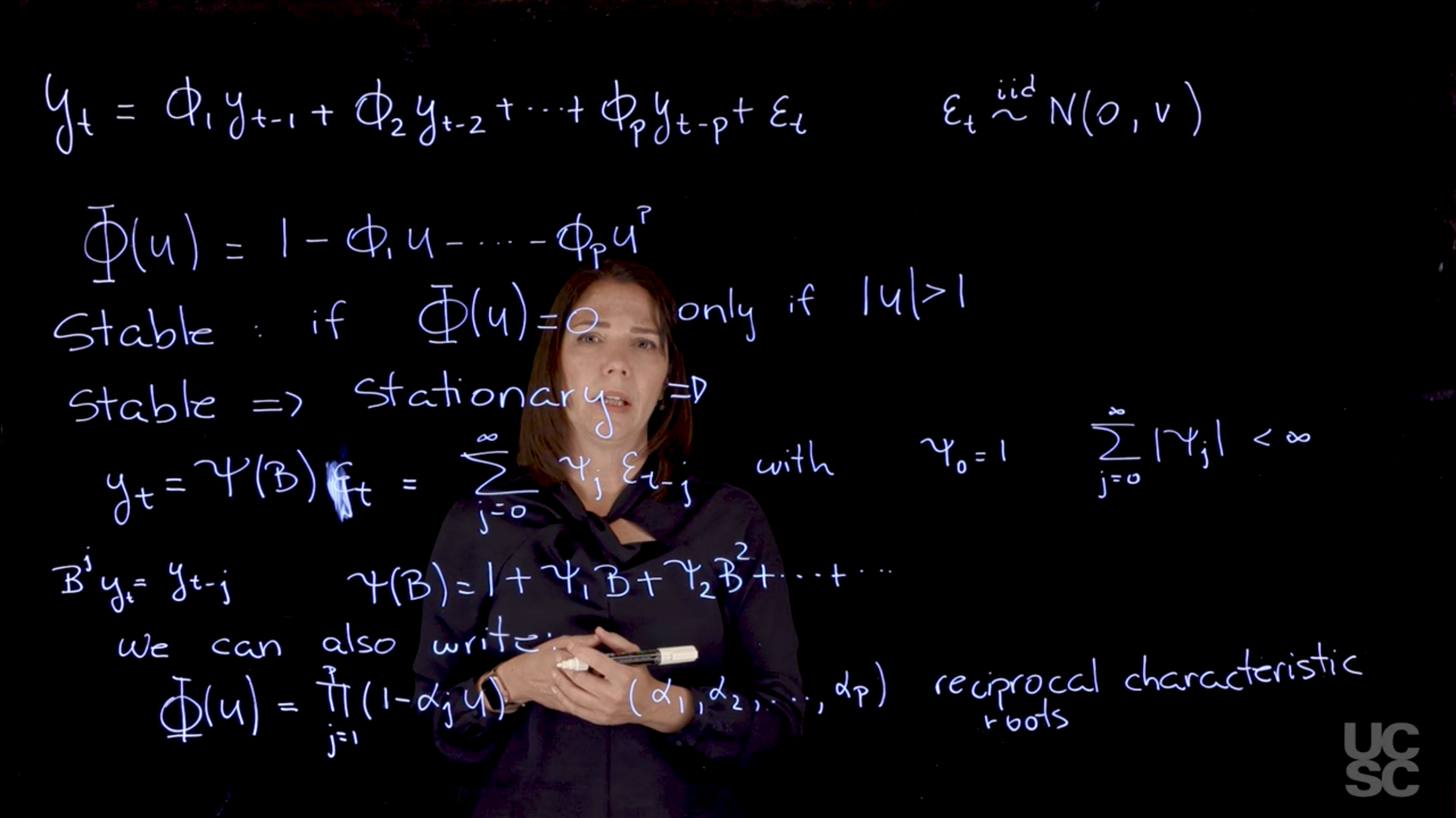
We will assume AR($p$) has the following structure:
$$
\textcolor{red}{y_t} = \textcolor{blue}{\phi_1} \textcolor{red}{y_{t-1}} + \textcolor{blue}{\phi_2} \textcolor{red}{y_{t-2}} + \ldots + \textcolor{blue}{\phi_p} \textcolor{red}{y_{t-p}} + \textcolor{grey}{\varepsilon_t}, \qquad \textcolor{grey}{\varepsilon_t} \overset{\text{iid}}{\sim} \mathcal{N}(0,v) \quad \forall t
$$ {#eq-ar-p-annotated}
where:
- $\textcolor{red}{y_t}$ is the value of the time series at time t
- $\textcolor{blue}{\phi_{1:p}}$ are the AR coefficients
- $\textcolor{grey}{\varepsilon_t} \overset{\text{iid}}{\sim} \mathcal{N}(0,v) \quad \forall t$ is a **white noise process** with zero mean and constant variance $v$.
### AR($p$) Characteristic Polynomial {#sec-arp-characteristic-polynomial}
A central outcome of the autoregressive nature of the **AR($p$)** is due to the properties the AR characteristic polynomial $\Phi$. [$\Phi$ AR characteristic polynomial]{.column-margin} This is defined as :
recall the backshift operator $B$ is defined as:
$$
\operatorname{B} y_t = y_{t-1}
$$
so that
$$
\operatorname{B}^j y_t = y_{t-j}
$$
We now use the backshift operator to rewrite the **AR($p$)** as a inhomogeneous linear difference equation:
$$
\begin{aligned}
y_t &= \phi_1 y_{t-1} + \phi_2 y_{t-2} + \ldots + \phi_p y_{t-p} + \varepsilon_t && \text{(AR($p$) defn.)} \newline
y_t &= \phi_1 \operatorname{B} y_t + \phi_2 \operatorname{B}^2 y_t + \ldots + \phi_p \operatorname{B}^p y_t + \varepsilon_t && \text{(B defn.)} \newline
\varepsilon_t &= y_t - \phi_1 \operatorname{B} y_t - \phi_2 \operatorname{B}^2 y_t - \ldots - \phi_p \operatorname{B}^p y_t && \text{(rearranging)} \newline
\varepsilon_t &= (1- \phi_1 \operatorname{B} - \phi_2 \operatorname{B}^2 - \ldots - \phi_p \operatorname{B}^p) y_t && \text{(factoring out $y_t$)}
\end{aligned}
$$ {#eq-ar-poly-derivation}
$$
\Phi(u) = 1 - \phi_1 u - \phi_2 u^2 - \ldots - \phi_p u^p \qquad \text{(Characteristic polynomial)}
$$ {#eq-ar-poly}
where:
- $u \in \mathbb{C}$ i.e. complex-valued roots
- $\phi_j$ are the AR coefficients.
::: {.callout-caution collapse="true"}
## Replacing the Backshift operator by Z {.unnumbered}
As far as the mathematics goes it isn't clear how we get from @eq-ar-poly-derivation to the characteristic polynomial $\Phi(z)$ in @eq-ar-poly.
As far as I can tell we can justify it by saying we have done three things:
1. We set $\varepsilon_t = 0$ to study the homogeneous equation. This is not about minimizing residuals but about analyzing the underlying linear recurrence, which governs the dynamics of the AR process without noise.
2. We assume $y_t \neq 0$. Since $\Phi(B)y_t = 0$, we can treat this as a linear operator equation. By analogy to polynomial equations, if $ab = 0$ and $b \neq 0$, then $a = 0$. Thus, we analyze the operator polynomial $\Phi(B) = 0$ as the condition for nontrivial solutions.
3. We replace the backshift operator $B$ with a complex number $z$, leading to the characteristic polynomial $\Phi(z)$:
- This is justified by assuming exponential solutions of the form $y_t = z^t$, a standard method in solving linear recurrences. Substituting into $\Phi(B)y_t = 0$ yields $\Phi(z^{-1}) = 0$, which we often rewrite as $\Phi(z) = 0$ for convenience.
- Alternatively, we view $B$ as a placeholder in a polynomial ring of operators, and replacing $B$ by $z$ evaluates that polynomial. This is a standard algebraic move in analyzing recurrence relations or z-transforms.
- Another point is that the backshift operator $B$ is just a linear operator on the space of time series. I.e it can be viewed as a matrix that shifts the time series back by one step.
:::
Diving a little deeper $\operatorname{B}$ is represented by a nilpotent matrix, which is a matrix that shifts the time series back by one step. This is a standard algebraic move in analyzing recurrence relations or z-transforms.
$$
B = \begin{pmatrix}
0 & 0 & 0 & \cdots & 0 \\
1 & 0 & 0 & \cdots & 0 \\
0 & 1 & 0 & \cdots & 0 \\
\vdots & \vdots & \vdots & \ddots & \vdots \\
0 & 0 & 0 & \cdots & 1
\end{pmatrix}
$$ {#eq-ar-poly-b-matrix}
This matrix is nilpotent because if you multiply it by itself enough times, it will eventually become the zero matrix. This is a key property that allows us to define the characteristic polynomial in terms of the backshift operator.
Note: that the above derivation wasn't presented in the slides but is my own attempt to clarify the steps involved I hope it is helpful not 100% sure it is correct.
- [This polynomial and its roots tells us a lot about the process and its properties. One of the main characteristics is it allows us to think about things like **quasi-periodic behavior**, whether it's present or not in a particular **AR($p$)** process. ]{.mark}
- It allows us to think about whether a process is **stationary or not**, depending on some properties related to this polynomial.
- In particular, we are going to say that the process is **stable** if all the roots of the characteristic polynomial have a modulus greater than one. [stability condition]{.column-margin}
> Why are we interested in this autoregressive lag polynomial?
$$
\Phi(z) = 0 \iff |z| > 1 \qquad \text{(stability condition)}
$$ {#eq-arp-stability}
- For any of the roots, it has to be the case that the modulus of that root, they have to be all outside the unit circle.
- If a process is stable, it will also be stationary.
We can show this as follows:
[If the AR($p$) has all the roots of its characteristic polynomial outside the unit circle, it is *stable* and *stationary* and can be written in terms of an infinite order *moving average* process:]{.mark}
$$
y_t = \Psi(\operatorname{B}) \varepsilon_t = \sum_{j=0}^{\infty} \psi_j \varepsilon_{t-j} \quad \text {with} \ \psi_0 = 1 \quad \text{ and } \sum_{j=0}^{\infty} |\psi_j| < \infty
$$ {#eq-ar-stationary}
where:
- $\varepsilon_t$ is a white noise process with zero mean and constant variance $v$.
- $\operatorname{B}$ is the lag operator AKA the backshift operator defined by $\operatorname{B} \varepsilon_t = \varepsilon_{t-1}$.
This need to be applied to a time series $\varepsilon_t$ to get the lagged values.
- $\Psi(\operatorname{B})$ is the infinite order polynomial in $\operatorname{B}$ that represents a linear filter applied to the noise process.
- $\psi_t = 1$ is the weight for the white noise at time $t$.
- the constraint $\psi_0 = 1$ ensures that the current shock contributes directly to $y_t$
- the constraint on the weights $\sum_{j=0}^{\infty} |\psi_j| < \infty$ ensures that the weights decay sufficiently fast, so that the process does not explode making it is stable and therefore stationary.
::: {.callout-caution collapse="true"}
### Notation Confusion {.unnumbered}
the notation with $\psi$ a functional of operator $B$ and $\psi_i$ as constants is confusing in both the reuse if the symbol and the complexity.
:::
We can also rewrite the characteristic polynomial in terms of the reciprocal roots of the polynomial.
The zeros of the characteristic polynomial are the roots of the **AR($p$)** process.
$$
\Phi(u) = \prod_{j=1}^{p} (1 - \alpha_j u) = 0 \implies u = \frac{1}{ \alpha_j} \qquad \text{(reciprocal roots)}
$$ {#eq-ar-p-reciprocal-roots}
where:
- $\alpha_j$ are the reciprocal roots of the characteristic polynomial.
Here, $u$ is any complex valued number.
<!--
Prado says we will show later .... where this roots have important properties.
It would be nice to state this explicitly and linked to the appropriate sections.
-->
### State Space Representation of AR($p$) {#sec-state-space-ar-p}
{#fig-ar-p-state-space .column-margin group="slides" width="53mm"}
This material is covered in [@prado2000bayesian § 2.1.2]
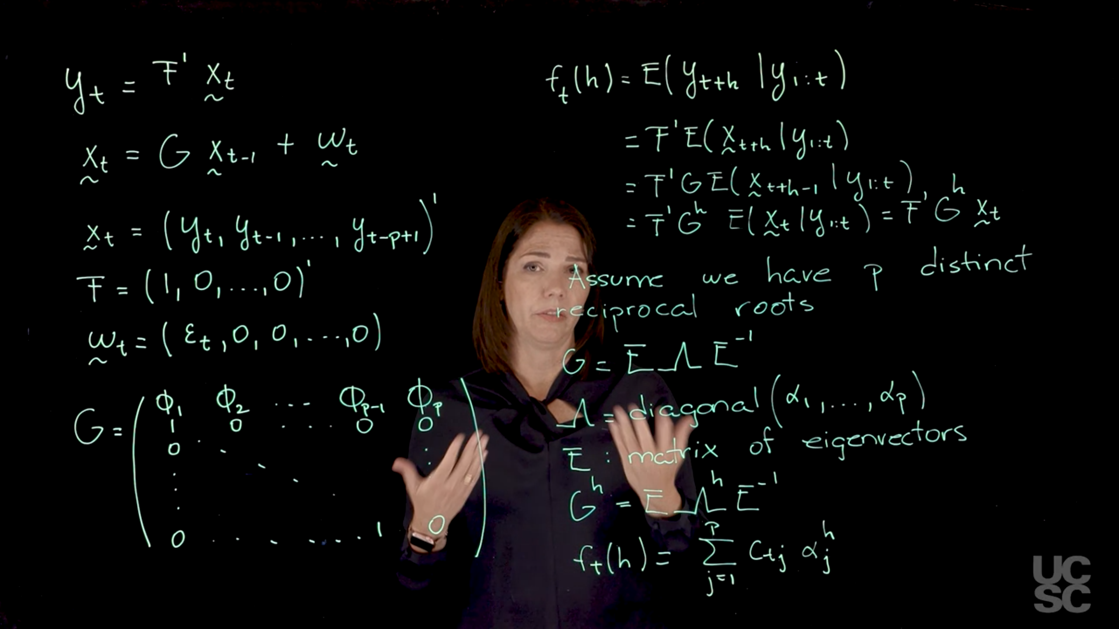
[Another important representation of the AR($p$) process, is based on a state-space representation of the process. This representation is useful because it allows us to study some important properties of the process.]{.mark} We will make some connections with these representations later when we talk about dynamic linear models, is given as follows for an AR($p$).
$$
y_t = \operatorname{F}^\top \mathbf{x}_t \qquad \text{(observational equation)}
$$ {#eq-state-space-observational-equation}
where:
- $\operatorname{F}$ is a linear mapping from the state space into the state space, so it is just vector of coefficients, specifically $F = (1, 0, \ldots, 0)^\top$ for the AR($p$) process. The rank for this operator is $p$ since it has to match the dimension of the state vector $\mathbf{x}_t$.
- $\mathbf{x}_t$ is a vector with the state of the process at time $t$.
To demystify $\operatorname{F}$, it is just picking the current state from vector $\mathbf{x}_t$ with states for the p previous time steps.
$$
\mathbf{x}_t = G \mathbf{x}_{t-1} + \mathbf{w}_t \qquad \text{(state equation)}
$$ {#eq-state-space-state-equation}
where:
- $\mathbf{x}_t$ is a vector of the current state of the process.
- $G$ is a state transition matrix that describes the relationship between the current state and the previous state.
- $\mathbf{x}_{t-1}$ is a vector of the previous state of the process.
- $\mathbf{w}_t$ is a vector of *innovations* or noise at time $t$, which is assumed to be normally distributed with zero mean and constant variance. The first component is going to be the $\varepsilon_t$ and the rest of the components are going to be zero and the dimension of this vector is going to be $p$.
\index{AR($p$)!state transition matrix}
and state transition matrix G
The $G$ matrix in this representation is going to be a very important matrix, the first row is going to contain the AR parameters, the AR coefficients, and we have $p$ of those. In the block below this is an identity matrix, and a zero column on it's right.
$$
G = \begin{pmatrix}
\phi_1 & \phi_2 & \phi_3 & \dots & \phi_{p-1} & \phi_p \\
1 & 0 & 0 & \dots & 0 & 0 \\
0 & 1 & 0 & \dots & 0 & 0 \\
\vdots & \ddots & \ddots & \ddots & & \vdots \\
0 & 0 & 0 & \dots & 1 & 0
\end{pmatrix}.
$$ {#eq-ar-p-state-space-g-matrix}
This state transition matrix $\mathbf{G}$ is important because it is related to the characteristic polynomial, in particular, is related to the reciprocal roots representation of the characteristic polynomial that we discussed before.
The structure of this $\mathbf{G}$ matrix is such that it captures the Markovian dynamics of the autoregressive process, wherein each $\mathbf{x}_t$ is a function of $\mathbf{x}_{t-1}$.
The eigenvalues of this matrix correspond precisely to the reciprocal roots of the characteristic polynomial.
Prado points out that if you perform the matrix operations described in @eq-state-space-observational-equation and @eq-state-space-state-equation, you will recover the form of your autoregressive process from the definition in @eq-ar-p-annotated .
So we have given the state-space representation of an AR($p$). One advantage of working with this representation is that we can use with it some definitions that apply to dynamic linear models or state-space models. One such definition is the so-called forecast function.
### The forecast function of AR($p$) {#sec-forecast-function-ar-p}
\index{AR($p$)!forecast function}
The forecast function, which we denote as $f_t(h)$ is a function $f$ that depends on the time $t$ that you're considering, and then you're looking at forecasting $h$ steps ahead in your time series.
If you have observations up to today and you want to look at what is the forecast function five days later, we will set $h=5$ there. The forecast function is just the expected value and we can just think of this as the expected value of $y_{t+h}.$ conditional on all the observations or all the information you have received up to time $t$.
$$
\begin{aligned}
f_t(h) &= \mathbb{E}[y_{t+h} \mid y_{1:t}] &\text{(defn)}\\
&= \mathbf{F}^\top \mathbb{E}[\mathbf{x}_{t+h} \mid y_{1:t}] &\text{(observation eq.)} \\
&= \mathbf{F}^\top \mathbf{G} \mathbb{E}[\mathbf{x}_{t+h-1} \mid y_{1:t}] &\text{(state eq.)} \\
&= \mathbf{F}^\top \mathbf{G}^h \mathbb{E}[\mathbf{x}_t\mid y_{1:t}], & \text{(repeat)} \\
&= \mathbf{F}^\top \mathbf{G}^h \mathbf{x}_t & h > 0, \forall t \ge p
\end{aligned}
$$ {#eq-ar-p-forecast-function-derivation}
where:
- $y_{1:t}$ is the vector of all observations up to time $t$,
- $\mathbf{x}_t$ is the state vector at time $t$.
- $\mathbf{G}^h$ is the state transition matrix raised to the power $h$, which captures the dynamics of the AR process over $h$ steps ahead. The eigenvalues of this matrix are the reciprocal roots of the characteristic polynomial of the AR($p$) process.
- In this derivation:
- We start with the expectation and rewrite it expectation using the state-space representation equations:
- We start using the observation equation, replacing $y_{t+h}$ with $F^T(\mathbf x_{t+h})$ in that case.
- Next we apply the second (state) equation.
- This introduces $\mathbf{G}$
- and updates our expected value to the next time step, so we have $\mathbf{X}_{t+h-1}$.
- Note: that since the $w_{t+h-1}$ terms are independent of the past observations, their expected value is zero, so we can leave them out.
- We repeat applying the state equation for all the lags until we get to time $t$, ending up with a product of $h$ $\mathbf{G}$ matrices here, so we end up with $\mathbf{G}^h$ and the each time we drop a lag in the expectation of $\mathbf{X}_{t+h}$.
- We end up with the expected value of $\mathbb{E}[\mathbf{x}_t]$ which is just the vector $\mathbf{x}_t$ the current state of the process.
This result is significant because it now allows us to make the connection of $\mathbf{G}$ and its eigenstructure. One of the features of $\mathbf{G}$ is that the eigenstructure is related to the reciprocal roots of the characteristic polynomial. So when we working with the case in which we have exactly p distinct roots. We can further simplify using by rewriting $\mathbf{G}$ in terms of its eigendecomposition.
We can rewrite $\mathbf{G}$ as $\mathbf{E}$, a matrix $\mathbf{\Lambda}$ here, $\mathbf{E}^{-1}$.
$$
\mathbf{G}= \mathbf{E} \mathbf{\Lambda} \mathbf{E}^{-1} \qquad \text{(eigendecomposition)}
$$ {#eq-ar-p-g-eigendecomposition}
where:
- $\mathbf{\Lambda} = \operatorname{diag}(\alpha_1, \ldots, \alpha_p)$ is a diagonal matrix consisting of the reciprocal roots $\alpha_i$, from the reciprocal formulation of the characteristic polynomial in @eq-ar-p-reciprocal-roots.
- While the order of the roots doesn't matter but there is a tradition of order eigenvalues them in decreasing value and this can help us to **identify our model**!
- $\mathbf{E}$ is a eigenvectors decomposition for the matrix $\mathbf{G}$
$E = [\mathbf{e}_1 ; \cdots ; \mathbf{e}_p]$, where $\mathbf{e}_i$ is the eigenvector corresponding to $\alpha_i$.
- Since each root is unique the eigenvectors are all different and linearly independent.
- Note that the eigendecomposition, i.e. the eigenvectors, has to follow the order set in $\Lambda$
We can now rewrite $\mathbf{G}^h$ as:
$$
\mathbf{G}^h= \mathbf{E} \mathbf{\Lambda}^h \mathbf{E}^{-1} \qquad \text{(eigendecomposition of G)}
$$ {#eq-ar-p-gh-eigendecomposition}
::: {.callout-caution collapse="true"}
### Why arn't the eigendecomposition powered up {.unnumbered}
So here is an easy answer
if $\mathbf{G}= \mathbf{E} \mathbf{\Lambda} \mathbf{E}^{-1}$
if we multiply out the all the $E$ and $E^{-1}$ terms cancel out except the last and first.
:::
Whatever elements have in the matrix of eigenvectors $\mathbf{E}$, they are now going to be functions of the reciprocal roots $u_i=\frac{1}{\phi_j}$.
The power that appears here, which is the number of steps ahead that you want to forecast in your time series for prediction,
$$
f_t(h) = E(y_{t+h} \mid y_{1:t}) = F^\top G^h x_t, \quad h > 0, \quad \forall t \ge p
$$ {#eq-ar-p-forecast-function}
where:
- $c_t$ are constants that depend on the $E$ matrix.
- $\alpha_i^h$ are the reciprocal roots raised to the power $h$.
We can see from the form of @eq-ar-p-forecast-function that if the process is stable, i.e. all the all the moduli of my reciprocal roots are going to be below one. So it is going to decay exponentially as a function of h. And this AR($p$) process is going to be stationary.
::: {.callout-important}
### Interpreting the forecast function {.unnumbered}
I recall that in physics we often view the eigenvectors as resonances of the system's dynamics, and the eigenvalues as the corresponding resonant frequencies. This is a good analogy to think about the reciprocal roots of the AR($p$) process. The contribution of each of the roots $\alpha_i$ to $f(t)$ depends on how close that modulus of that reciprocal root is to 1 or -1. For roots that have relatively large values of the modulus, then they are going to have more contribution in terms of what's going to happen in the future.
Depending on whether those reciprocal roots $\alpha_i$ are real-valued or complex-valued, you're going to have behavior here that may be quasiperiodic for complex-valued roots or just non-quasiperiodic for the real valued roots.
:::
In the text book AR($p$) forecasting is covered in [@prado2000bayesian § 2.2] and the mean square errors can be estimated using an algorithm by [@brockwell1991time].
<!-- TODO: summarize this transcript -->
::: {.callout-note collapse="true"}
## Video Transcript
{{< include transcripts/c4/02_week-2-the-ar-p-process/01_the-general-ar-p-process/01_definition-and-state-space-representation.en.txt >}}
:::
## Examples :movie_camera:
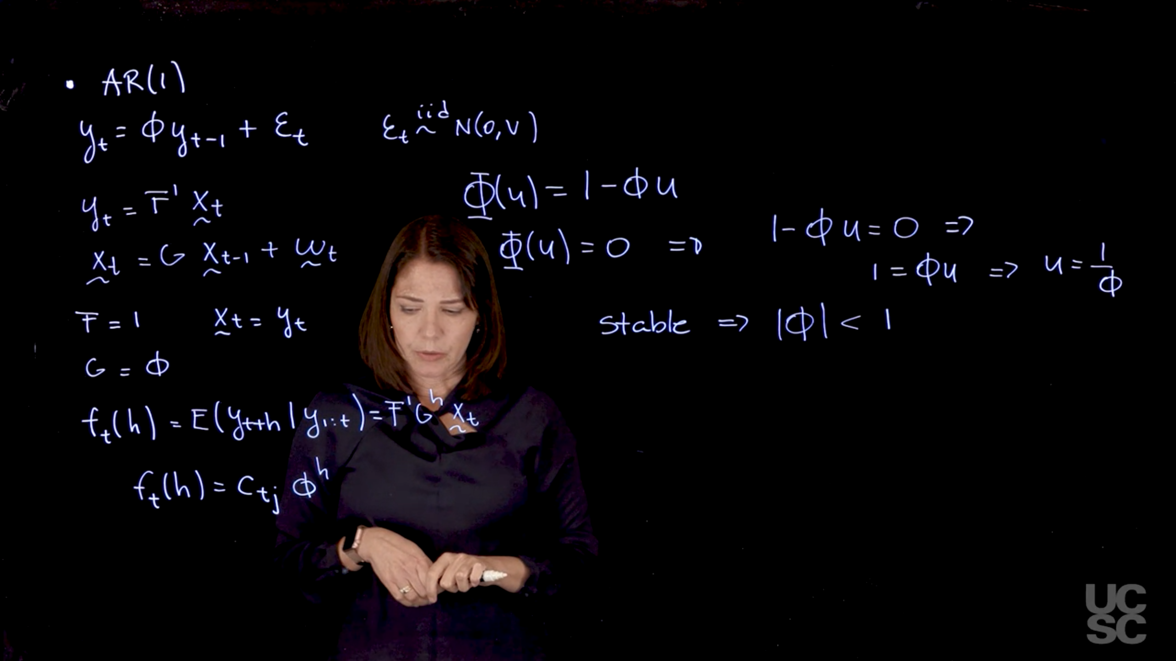
### **AR(1) Process**
{#fig-ar1-example .column-margin group="slides" width="53mm"}
* **State-space form**:
$X_t = \phi X_{t-1} + \omega_t$
* **Forecast function**:
$\mathbb{E}[y_{t+h} \mid \mathcal{F}_t] = c \cdot \phi^h$
* **Behavior**:
Exponential decay (oscillatory if $\phi < 0$), mimicking the autocorrelation function.
* **Stability**:
$|\phi| < 1$ (reciprocal root $1/\phi$ has modulus > 1).
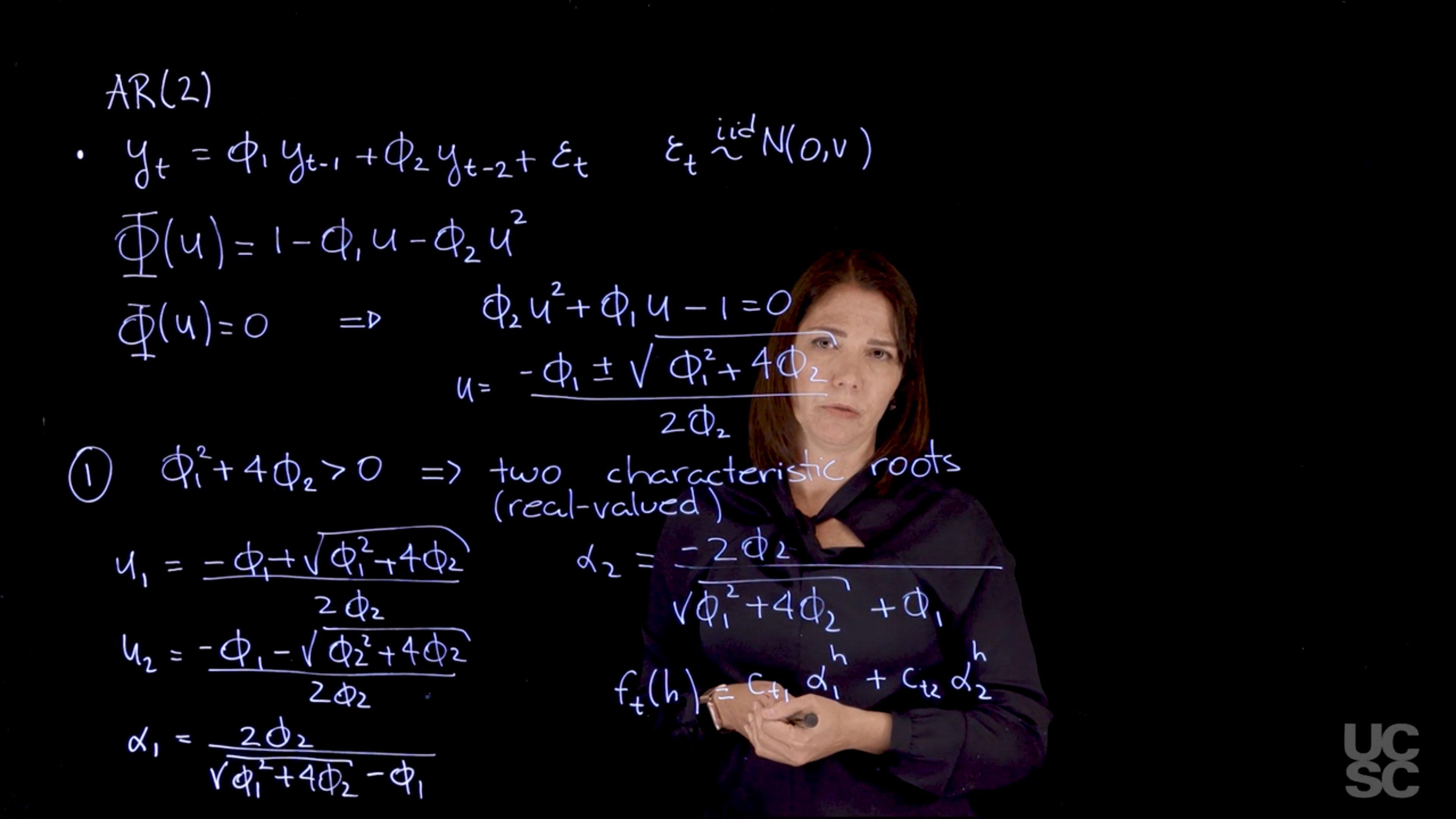
### **AR(2) Process**
{#fig-ar2-two-positive-roots .column-margin group="slides" width="53mm"}
{#fig-ar2-complex-roots .column-margin group="slides" width="53mm"}
* **Characteristic polynomial**: $1 - \phi_1 z - \phi_2 z^2$
* **Three root types**:
1. **Two real distinct reciprocal roots**:
Forecast function:
$$
\mathbb{E}[y_{t+h} \mid \mathcal{F}_t] = c_{t1} \alpha_1^h + c_{t2} \alpha_2^h
$$
Exponential decay, dominated by root with larger modulus.
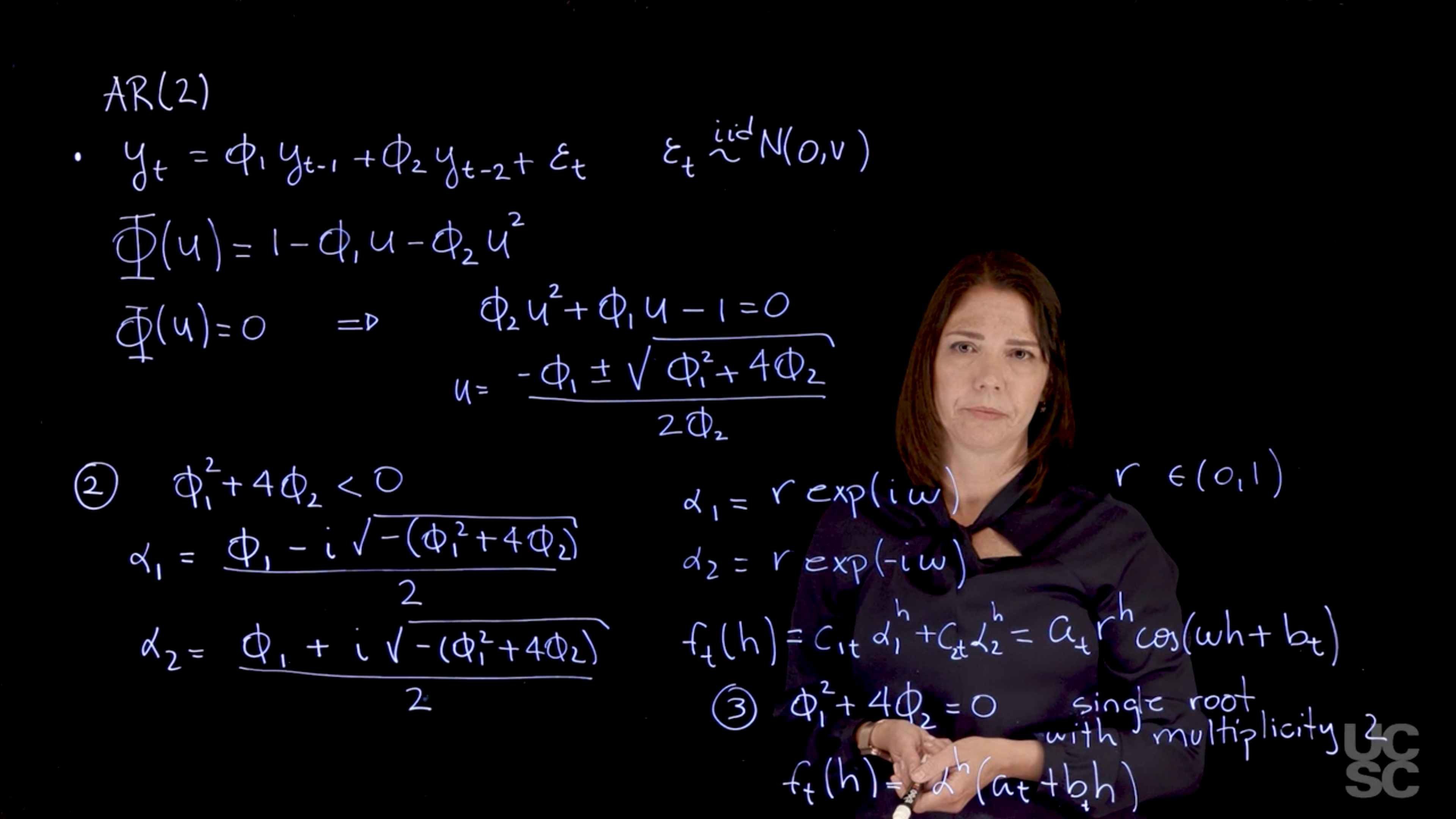
2. **Two complex conjugate reciprocal roots**: Let roots be $r e^{\pm i\omega}\$.
Forecast function:
$$
\mathbb{E}[y_{t+h} \mid \mathcal{F}_t] = A_t r^h \cos(\omega h + \delta_t)
$$
Behavior: *Quasiperiodic* with exponential envelope.
3. **Repeated reciprocal root (\$\alpha\$ with multiplicity 2)**:
Forecast function:
$$
\mathbb{E}[y_{t+h} \mid \mathcal{F}_t] = (\alpha^h)(a_t + b_t h)
$$
Polynomial-exponential form due to root multiplicity.
### Key Concepts
* Forecast structure mirrors the **roots** of the characteristic polynomial.
* Stability depends on **reciprocal roots** (modulus < 1).
* Complex roots → sinusoidal terms;
* Repeated roots → polynomial multipliers.
This analysis connects **forecast behavior** to the **algebraic properties** of AR model roots.
<!-- TODO: summarize this transcript -->
::: {.callout-note collapse="true"}
## Video Transcript
{{< include transcripts/c4/02_week-2-the-ar-p-process/01_the-general-ar-p-process/02_examples.en.txt >}}
:::
## ACF of the AR($p$) :movie_camera:
{#fig-acf-ar-p .column-margin group="slides" width="53mm"}
For a **stationary AR($p$)** process, the **autocorrelation function (ACF)** satisfies a homogeneous linear difference equation whose solution is a sum of terms involving the **reciprocal roots** of the characteristic polynomial. Key points:
* If there are $r$ distinct reciprocal roots $\alpha_1, \ldots, \alpha_r$ with multiplicities $m_1, \ldots, m_r$ such that $\sum m_j = p$, the ACF has the general form:
$$
\rho(h) = \sum_{j=1}^r P_j(h)\alpha_j^h,
$$
where each $P_j(h)$ is a polynomial of degree $m_j - 1$.
* For **distinct reciprocal roots** (common case), all $m_j = 1$, so $\rho(h)$ is a linear combination of powers of the roots.
* **AR(1)**: ACF is $\rho(h) = \phi^h$, where $\phi$ is the AR coefficient.
* **AR(2)**: Three cases arise:
1. Two distinct real roots → exponential decay.
2. Complex conjugate roots → **damped sinusoidal** behavior $r^h \cos(\omega h + \delta)$.
3. One real root with multiplicity 2 → decay with polynomial factor.
* ACF decays **exponentially** if all reciprocal roots lie inside the unit circle.
* The **Partial ACF (PACF)** of AR($p$) is **zero for all lags > p**.
* PACF values can be computed recursively via the **Durbin–Levinson algorithm**, using sample autocorrelations.
<!-- TODO: summarize this transcript -->
::: {.callout-note collapse="true"}
## Video Transcript
{{< include transcripts/c4/02_week-2-the-ar-p-process/01_the-general-ar-p-process/03_acf-of-the-ar-p.en.txt >}}
:::
## Simulating data from an AR($p$) :movie_camera:
This video goes through the code in the following sections, which simulates data from an AR($p$) process and plots the sample ACF and PACF.
1. **Characteristic Roots from AR Coefficients**:
* Given AR coefficients (e.g. for AR(8)), compute characteristic roots using `polyroot()` on the reversed sign polynomial (first term 1, followed by negative AR coefficients).
* Reciprocal roots are obtained as $1/\text{root}$.
* Use `Mod()` for modulus and $2\pi / \text{Arg}()$ for approximate periods of the reciprocal roots.
2. **Example AR(8)**:
* Yields 4 complex-conjugate pairs.
* Most persistent: modulus ≈ 0.97, period ≈ 12.7.
* Others show lower modulus and shorter periods, contributing less to persistence.
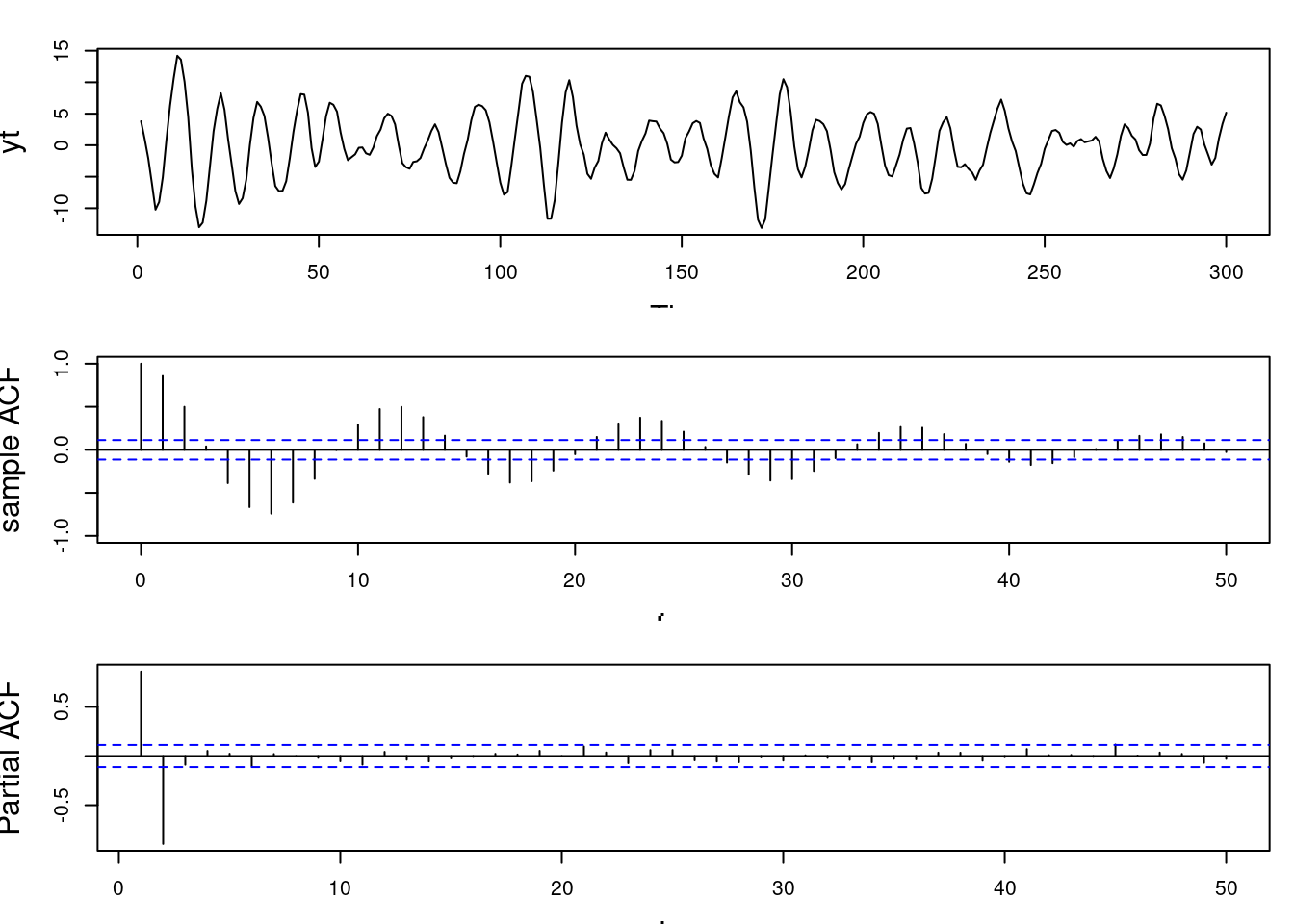
3. **Simulating AR(2) with Complex Roots**:
* Reciprocal root modulus 0.95, period 12 → converted to AR coefficients (≈ 1.65, -0.902).
* Simulated data shows quasi-periodic behavior.
* ACF: decaying sinusoidal pattern.
* PACF: significant at lags 1 and 2, then drops, consistent with AR(2).
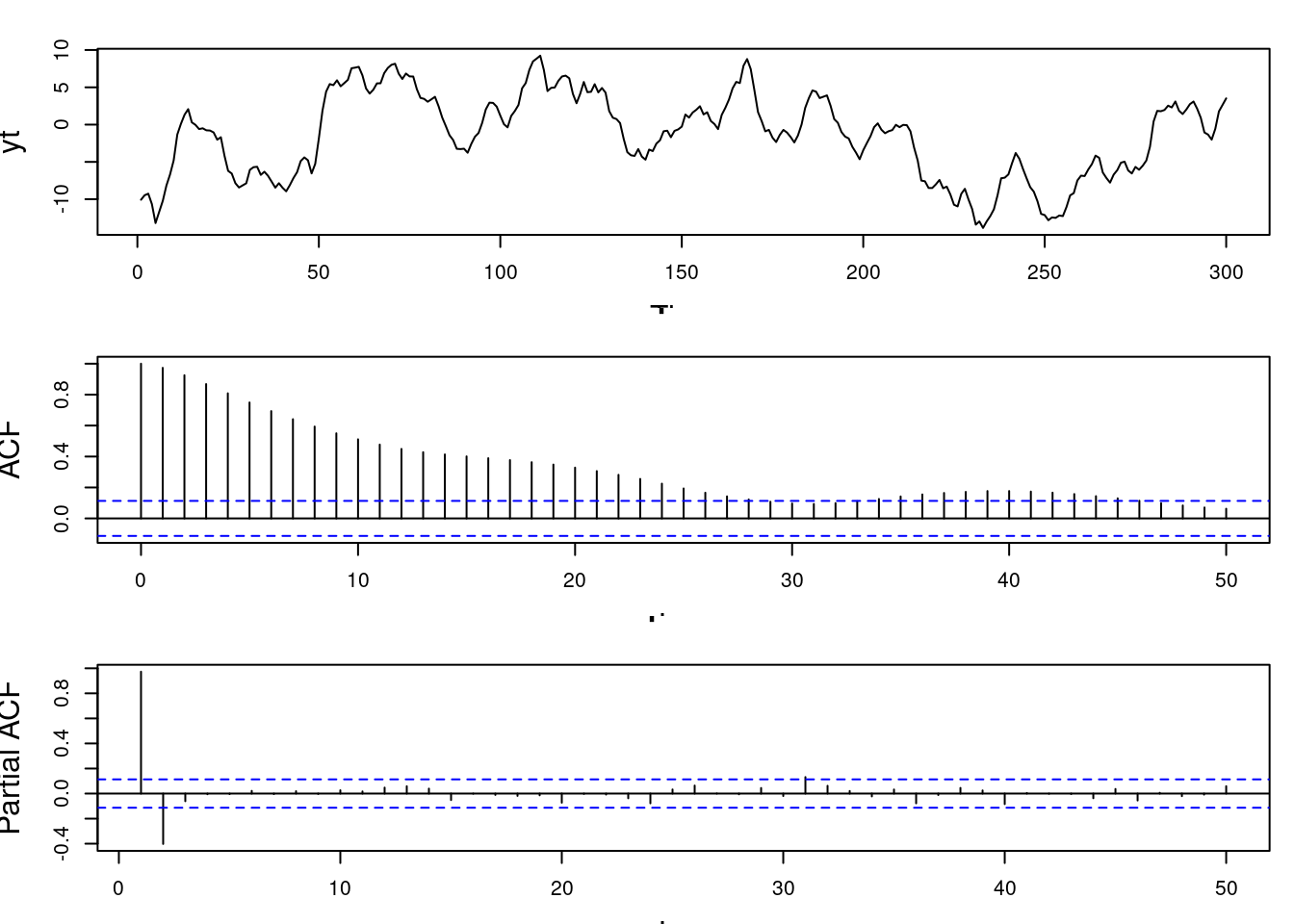
4. **Simulating AR(2) with Real Roots**:
* Roots: 0.95 and 0.5.
* AR coefficients derived from these.
* No quasi-periodic pattern in data; resembles damped random walk.
* ACF: smooth decay.
* PACF: only first two lags significant.
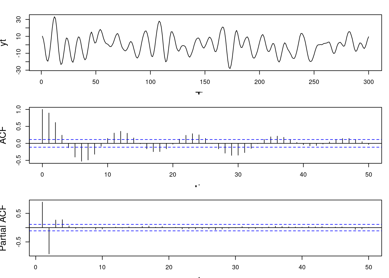
5. **Simulating AR(3) with Complex + Real Root**:
* Complex root pair: modulus 0.95, period 12; real root: modulus 0.8.
* Three AR coefficients derived.
* Simulated series shows quasi-periodic behavior plus extra persistence.
* ACF: still shows decaying periodicity.
* PACF: more than two significant lags, consistent with *AR(3)*.
**Key Insight**:
The modulus and type (real vs. complex) of reciprocal roots determine persistence and periodicity. The ACF reflects these traits, while the PACF helps identify AR order.
## Computing the roots of the AR polynomial :spiral_notepad: $\mathcal{R}$
Compute AR reciprocal roots given the AR coefficients
```{r}
#| label: lst-compute-ar-p-reciprocal-roots
#| list-label: lst-compute-ar-p-reciprocal-roots
#| list-caption: Compute AR reciprocal roots given the AR coefficients
# Assume the folloing AR coefficients for an AR(8)
phi=c(0.27, 0.07, -0.13, -0.15, -0.11, -0.15, -0.23, -0.14)
roots=1/polyroot(c(1, -phi)) # compute reciprocal characteristic roots
r=Mod(roots) # compute moduli of reciprocal roots
lambda=2*pi/Arg(roots) # compute periods of reciprocal roots

# print results modulus and frequency by decreasing order
print(cbind(r, abs(lambda))[order(r, decreasing=TRUE), ][c(2,4,6,8),])
```
<!-- TODO: summarize this transcript -->
::: {.callout-note collapse="true"}
## Video Transcript
{{< include transcripts/c4/02_week-2-the-ar-p-process/01_the-general-ar-p-process/04_simulating-data-from-an-ar-p.en.txt >}}
:::
## Simulating data from an AR($p$) :spiral_notepad: $\mathcal{R}$
\index{AR($p$)}
\index{ARIMA}
1. R code to simulate data from an AR(2) with one pair of complex-valued reciprocal roots and plot the corresponding sample ACF and sample PACF
```{r}
#| label: ar-sim-complex-valued-roots
## simulate data from an AR(2)
set.seed(2021)
## AR(2) with a pair of complex-valued roots with modulus 0.95 and period 12
r=0.95
lambda=12
phi=numeric(2)
phi[1]<- 2*r*cos(2*pi/lambda)
phi[2] <- -r^2
phi
T=300 # number of time points
sd=1 # innovation standard deviation
yt=arima.sim(n=T, model = list(ar = phi), sd=sd)

par(mfrow = c(3, 1), mar = c(3, 4, 2, 1), cex.lab = 1.5)
## plot simulated data
ts.plot(yt)
## draw sample autocorrelation function
acf(yt, lag.max = 50,
    type = "correlation", ylab = "sample ACF",
    lty = 1, ylim = c(-1, 1), main = " ")

## draw sample partial autocorrelation function
pacf(yt, lag.ma = 50, main = "sample PACF")
```
2. R code to simulate data from an AR(2) with two different real-valued reciprocal roots and plot the corresponding sample ACF and sample PACF
```{r}
#| label: ar-sim-real-valued-roots
### Simulate from AR(2) with two real reciprocal roots (e.g., 0.95 and 0.5)
set.seed(2021)
recip_roots=c(0.95, 0.5) ## two different real reciprocal roots
phi=c(sum(recip_roots), -prod(recip_roots)) ## compute ar coefficients
phi
T=300 ## set up number of time points
sd=1 ## set up standard deviation
yt=arima.sim(n=T,model = list(ar=phi),sd=sd) # generate ar(2)

par(mfrow = c(3, 1), mar = c(3, 4, 2, 1),  cex.lab = 1.5, cex.main = 1.5)
### plot simulated data
ts.plot(yt)
### plot sample ACF
acf(yt, lag.max = 50, type = "correlation",  main = "sample ACF")
### plot sample PACF
pacf(yt, lag.max = 50, main = "sample PACF")
```
3. R code to simulate data from an $AR(3)$ with one real reciprocal root and a pair of complex-valued reciprocal roots and plot the corresponding sample ACF and sample PACF
```{r}
#| label: ar-sim-ar3
### Simulate from AR(3) with one real root
### and a pair of complex roots (e.g., r=0.95 and lambda = 12 and real root with
### 0.8 modulus)
set.seed(2021)
r= c(0.95, 0.95, 0.8) ## modulus
lambda=c(-12, 12) ## lambda
recip_roots=c(r[1:2]*exp(2*pi/lambda*1i), r[3]) ## reciprocal roots
phi <- numeric(3) # placeholder for phi
phi[1]=Re(sum(recip_roots)) # ar coefficients at lag 1
phi[2]=-Re(recip_roots[1]*recip_roots[2] + recip_roots[1]*recip_roots[3] + recip_roots[2]*recip_roots[3]) # ar coefficients at lag 2
phi[3]=Re(prod(recip_roots))
phi
T=300 # number of time points
sd=1 # standard deviation
yt=arima.sim(n=T,model = list(ar=phi), sd = sd) # generate ar(3)

par(mfrow = c(3,1),  mar = c(3, 4, 2, 1), cex.lab = 1.5, cex.main = 1.5)
### plot simulated data
ts.plot(yt)
### plot sample ACF
acf(yt, lag.max = 50, type = "correlation",  main = "sample ACF")
### plot sample PACF
pacf(yt, lag.max = 50, main = "sample PACF")
```
## The AR($p$): Review :spiral_notepad: {#sec-arp-review}
This section is based on material from the [handout](handouts/c4-arp_summary.pdf) but we also covered it in greater detail at the beginning of the lecture.
### AR($p$): Definition, stability, and stationarity {#sec-arp-definition-stability-stationarity}
::: {.callout-info}
### AR($p$) {.unnumbered}
A time series follows a zero-mean autoregressive process of order $p$, of AR($p$), if:
$$
y_t = \phi_1 y_{t-1} + \phi_2 y_{t-2} + \ldots + \phi_p y_{t-p} + \varepsilon_t \qquad
$$ {#eq-ar-p}
where $\phi_1, \ldots, \phi_p$ are the AR coefficients and $\varepsilon_t$ is a white noise process
with $\varepsilon_t \sim \text{i.i.d. } N(0, v)$, for all $t$.
:::
The AR characteristic polynomial is given by
$$
\Phi(u) = 1 - \phi_1 u - \phi_2 u^2 - \ldots - \phi_p u^p,
$$
with $u$ complex-valued.
The AR($p$) process is stable if $\phi(u) = 0$ only when $\|u\| > 1$. In this case, the process is also stationary and can be written as
$$
y_t = \psi(B) \varepsilon_t = \sum_{j=0}^{\infty} \psi_j \varepsilon_{t-j},
$$
with $\psi_0 = 1$ and $\sum_{j=0}^{\infty} |\psi_j| < \infty$. Here $B$ denotes the backshift operator, so $B^j \varepsilon_t = \varepsilon_{t-j}$ and
$$
\psi(B) = 1 + \psi_1 B + \psi_2 B^2 + \ldots + \psi_j B^j + \ldots
$$
The AR polynomial can also be written as
$$
\Phi(u) = \prod_{j=1}^{p} (1 - \alpha_j u),
$$
with $\alpha_j$ being the reciprocal roots of the characteristic polynomial. For the process to be stable (and consequently stationary), $|\alpha_j| < 1$ for all $j = 1, \ldots, p$.
### AR($p$): State-space representation {#sec-arp-state-space-representation}
An AR($p$) can also be represented using the following state-space or dynamic linear (DLM) model representation:
$$
y_t = F^{\top} x_t,
$$ {#eq-ar-p-state-space-y}
$$
x_t = G x_{t-1} + \omega_t,
$$ {#eq-ar-p-state-space-x}
with
$$
x_t = (y_t, y_{t-1}, \dots, y_{t-p+1})^{\top}
$$ {#eq-ar-p-state-space-x-vector}
where F is a mapping from the state vector to the observed variable:
$$
F = (1, 0, \dots, 0)^{\top}
$$ {#eq-ar-p-state-space-f-vector}
$$
\omega_t = (\varepsilon_t, 0, \dots, 0)^{\top}
$$ {#eq-ar-p-state-space-omega-vector}
\index{AR($p$)!state transition matrix}
and state transition matrix G
$$
G = \begin{pmatrix}
\phi_1 & \phi_2 & \phi_3 & \dots & \phi_{p-1} & \phi_p \\
1 & 0 & 0 & \dots & 0 & 0 \\
0 & 1 & 0 & \dots & 0 & 0 \\
\vdots & \ddots & \ddots & \ddots & & \vdots \\
0 & 0 & 0 & \dots & 1 & 0
\end{pmatrix}.
$$ {#eq-ar-p-state-space-g-matrix}
\index{AR($p$)!forecast function}
Using this representation, the expected behavior of the process in the future can be exhibited via the forecast function:
$$
f_t(h) = E(y_{t+h} \mid y_{1:t}) = F^\top G^h x_t, \quad h > 0, \quad \forall t \ge p
$$ {#eq-ar-p-forecast-function}
Where $G^h$ is the $h$^-th^ power of the matrix $G$.
The eigenvalues of the matrix $G$ are the reciprocal roots of the characteristic polynomial.
::: {.callout-note}
### Eigenvalues {.unnumbered}
- The eigenvalues can be real-valued or complex-valued.
- If they are Complex-valued the eigenvalues/reciprocal roots appear in conjugate pairs.
:::
Assuming the matrix $G$ has $p$ distinct eigenvalues, we can decompose $G$ into $G = E \Lambda E^{-1}$, with
$$
\Lambda = \text{diag}(\alpha_1, \dots, \alpha_p),
$$
for a matrix of corresponding eigenvectors $E$. Then, $G^h = E \Lambda^h E^{-1}$ and we have:
$$
f_t(h) = \sum_{j=1}^{p} c_{tj} \alpha_j^h.
$$
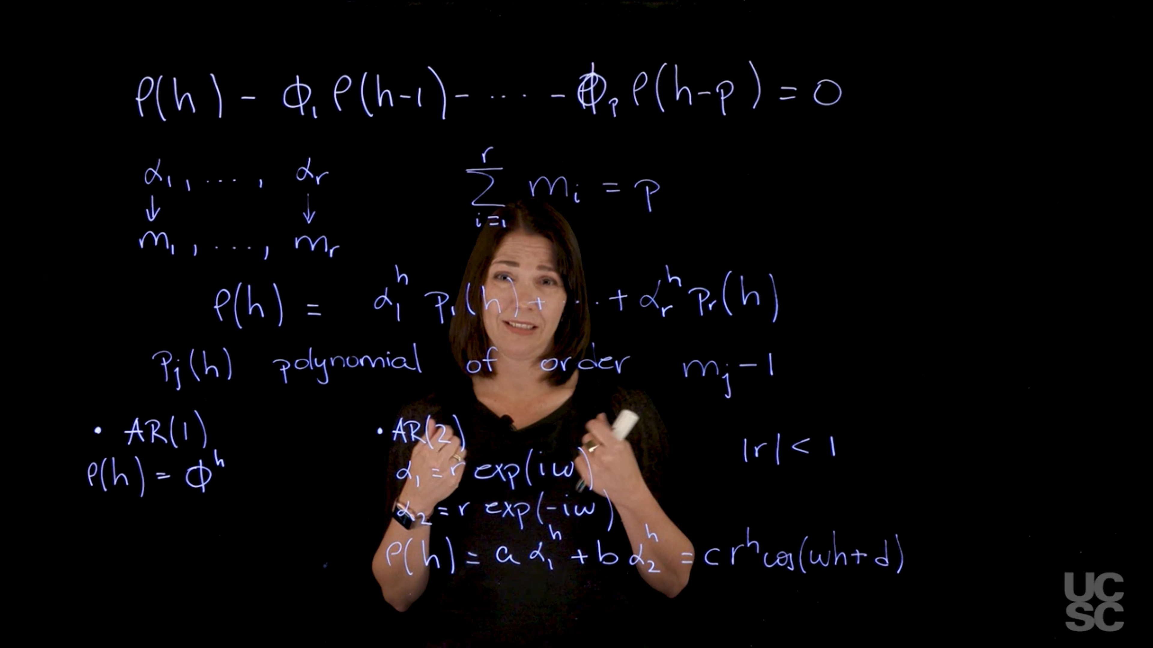
### ACF of AR($p$) {#sec-arp-acf}
For a general AR($p$), the ACF is given in terms of the homogeneous difference equation:
$$
\rho(h) - \phi_1 \rho(h-1) - \ldots - \phi_p \rho(h-p) = 0, \quad h > 0.
$$
Assuming that $\alpha_1, \dots, \alpha_r$ denotes the characteristic reciprocal roots each with multiplicity $m_1, \ldots, m_r$, respectively, with $\sum_{i=1}^{r} m_i = p$. Then, the general solution is
$$
\rho(h) = \alpha_1^h p_1(h) + \ldots + \alpha_r^h p_r(h),
$$
with $p_j(h)$ being a polynomial of degree $m_j - 1$.
### Example: AR(1) {#sec-arp-example-ar1}
We already know that for $h \ge 0$, $\rho(h) = \phi^h$. Using the result above, we have
$$
\rho(h) = a \phi^h,
$$
and so to find $a$, we take $\rho(0) = 1 = a \phi^0$, hence $a = 1$.
### Example: AR(2) {#sec-arp-example-ar2}
Similarly, using the result above in the case of two complex-valued reciprocal roots, we have
$$
\rho(h) = a \alpha_1^h + b \alpha_2^h = c r^h \cos(\omega h + d).
$$
### PACF of AR($p$) {#sec-arp-pacf}
\index{PACF}
\index{AR($p$)!PACF}
\index{Durbin-Levinson}
We can use the **Durbin-Levinson recursion** to obtain the PACF of an AR($p$). c.f. @sec-durbin-levinson.
Using the same representation but substituting the true **autocovariances** and **autocorrelations** with their sampled versions, we can also obtain the **sample PACF**.
It is possible to show that the PACF of an AR($p$) is equal to zero for $h > p$.