---
title: "Distributions - M1L3"
subtitle: "Bayesian Statistics: From Concept to Data Analysis"
subject: "Bayesian Statistics"
description: "Outline of distributions"
categories:
- Bayesian Statistics
keywords:
- Distributions
- Bernoulli Distribution
- Binomial Distribution
---
## Distributions {#sec-distributions}
```{python}
#| echo: false
#import pandas as pd
```
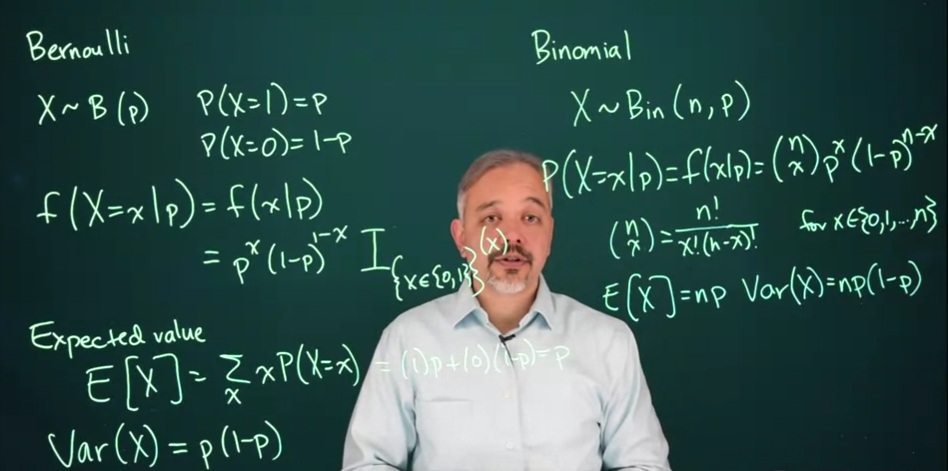
## The Bernoulli & Binomial Distribution {#sec-the-bernoulli--binomial-distribution}
{#fig-slide-l03-s01 .column-margin width="53mm" group="slides"}
These two distributions are built on a trial of a coin toss (possibly biased).
- We use the Bernoulli distribution to model a random variable for the probability of such a coin toss trial.
- We use the Binomial distribution to model a random variable for the probability of getting $k$ heads in $N$ independent trials.
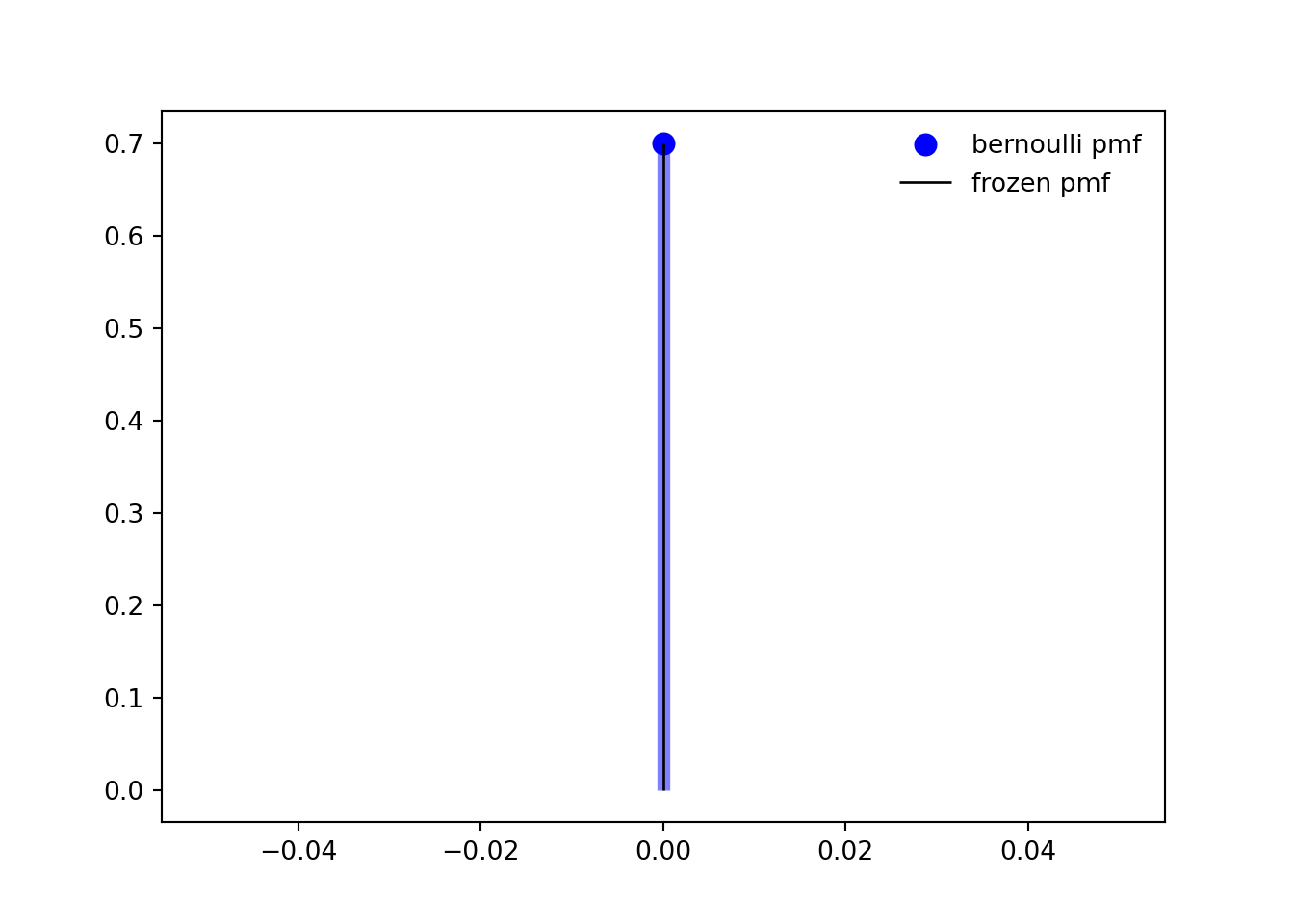
### The Bernoulli Distribution {#sec-the-bernoulli-distribution}
Arises when modeling events with two possible outcomes, **Success** and **Failure** for a coin toss these can be **Heads** and **Tails**
```{r include=FALSE}
# Necessary for using dvisvgm on macOS
# See https://www.andrewheiss.com/blog/2021/08/27/tikz-knitr-html-svg-fun/
Sys.setenv(LIBGS = "/usr/local/share/ghostscript/9.53.3/lib/libgs.dylib.9.53")
font_opts <- list(dvisvgm.opts = "--font-format=woff")
```
$$
X \sim \mathrm{Bernoulli}(p) =
\begin{cases}
\mathbb{P}r(X=1) = p & \text{success} \\
\mathbb{P}r(X=0)=1-p & \text{failure}
\end{cases}
$$ {#eq-l3-bernoulli-rv}
Where parameter p is the probability of getting heads.
The probability for the two events is:
Notation:
- we use (Roman) p if its value is known.\
- we use (Greek) $\theta$ when its value is unknown.
This is a probability mass function since it is discrete. But we call it a Probability Density Function (PDF) in the measure-theoretic sense.
$$
f(X=x\mid p) = p^x(1-p)^x \mathbb{I}_{[0,1]}(x)
$$ {#eq-l3-bernoulli-pmf}
$$
\mathbb{E}(x)= p
$$ {#eq-l3-bernoulli-expectation}
$$
\text{Var}(x)= \mathbb{P}r(1-p)
$$ {#eq-l3-bernoulli-variance}
```{python}
#| label: "bernoulli-distribution"
#| fig-cap: "Bernoulli distribution"
import numpy as np
from scipy.stats import bernoulli
import matplotlib.pyplot as plt

fig, ax = plt.subplots(1, 1)
p = 0.3
mean, var, skew, kurt = bernoulli.stats(p, moments='mvsk')
print(f'{mean=:1.2f}, {var=:1.2f}, {skew=:1.2f}, {kurt=:1.2f}')
x = np.arange(bernoulli.ppf(0.01, p),
              bernoulli.ppf(0.99, p))
ax.plot(x, bernoulli.pmf(x, p), 'bo', ms=8, label='bernoulli pmf')
ax.vlines(x, 0, bernoulli.pmf(x, p), colors='b', lw=5, alpha=0.5)

rv = bernoulli(p)
ax.vlines(x, 0, rv.pmf(x), colors='k', linestyles='-', lw=1,
        label='frozen pmf')
ax.legend(loc='best', frameon=False)
plt.show()
## Generate random numbers
r = bernoulli.rvs(p, size=10)
r
```
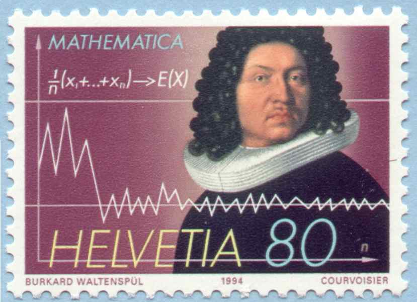{#fig-bio-bernoulli .column-margin width="53mm" group="slides"}
::: {.callout-tip}
### Biographical note on Jacob Bernoulli
> It seems that to make a correct conjecture about any event whatever, it is necessary to calculate exactly the number of possible cases and then to determine how much more likely it is that one case will occur than another. [@bernoulli1713ars]
The Bernoulli distribution as well as The Binomial distribution are due to Jacob Bernoulli (1655-1705) who was a prominent mathematicians in the Bernoulli family. He discovered the fundamental mathematical constant e. However, his most important contribution was in the field of probability, where he derived the first version of the law of large numbers.
for a fuller [biography see](https://mathshistory.st-andrews.ac.uk/Biographies/Bernoulli_Jacob/)
:::
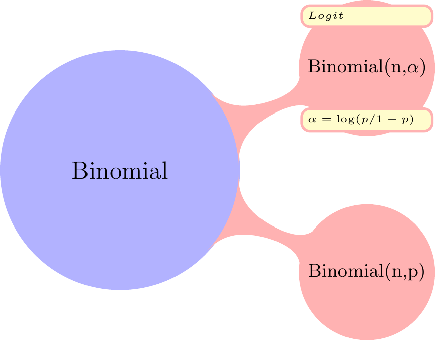
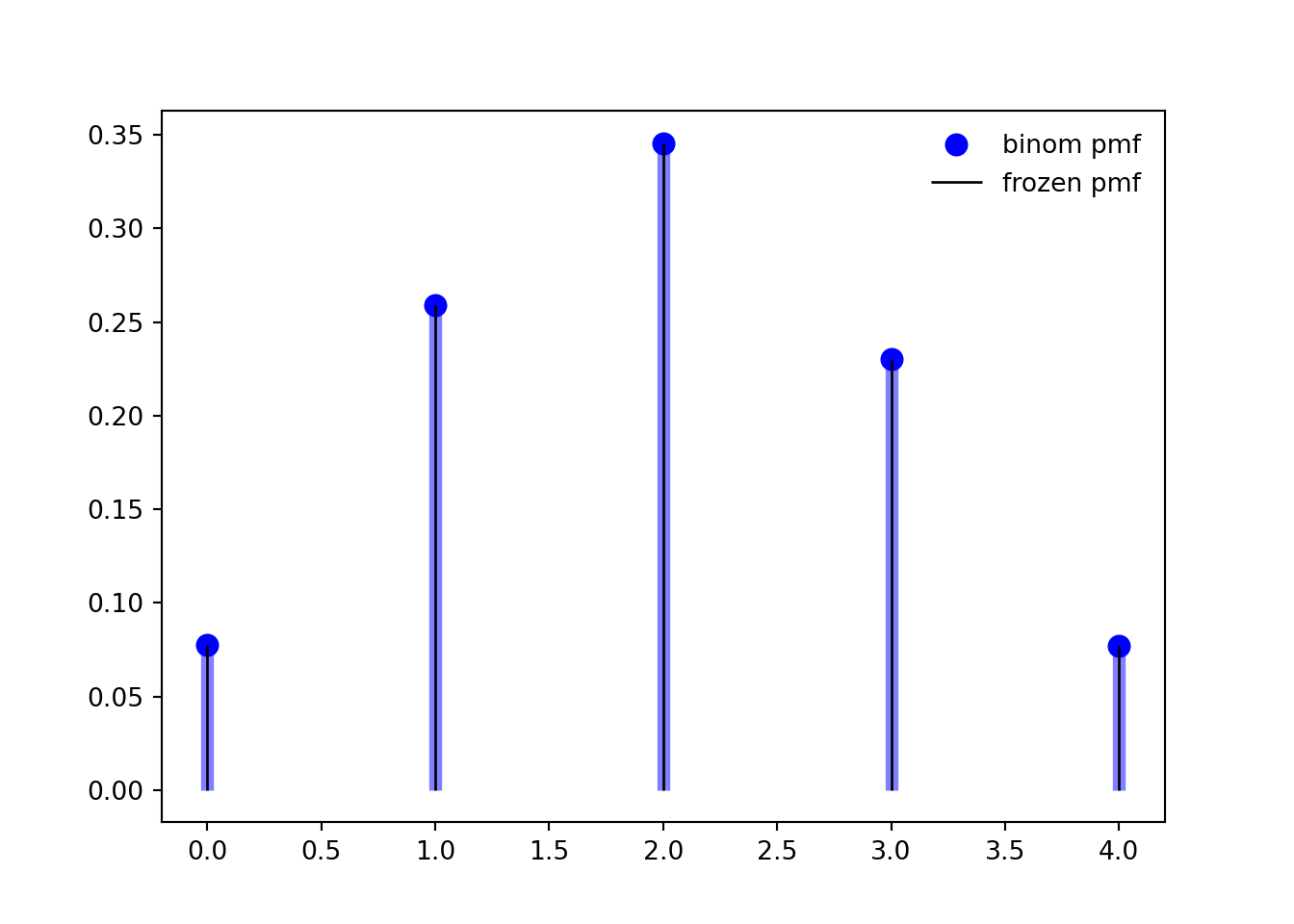
### The Binomial Distribution
$$
\overbrace{\underbrace{\fbox{0}\ \ldots \fbox{0}}_{N_0}\ \underbrace{\fbox{1}\ \ldots \fbox{1}}_{N_1}}^N
$$ {#eq-l3-bernoulli-experiment}
The Binomial distribution models `counts` of successes in independent Bernoulli trials \index{Bernoulli trial}. It arises when we need to consider the summing N independent and identically distributed Bernoulli RV with the same probability of success $\theta$.
::: {.callout-tip}
#### Conditions
- Discrete data
- Two possible outcomes for each trial
- Each trial is independent
- The probability of success/failure is the same in each trial
:::
```{tikz Binomial-reparams, engine.opts=font_opts}
#| echo: false
#| fig-cap: "Binomial reparams mindmap"
#| fig-align: center
#| fig-ext: png
#| out-width: 100%
\usetikzlibrary {mindmap,backgrounds,calc}
\begin{tikzpicture}[
mindmap,
concept color=red!30,
every node/.style = {concept},
grow cyclic,
level 1/.append style = {
level distance = 4.5cm,
sibling angle = 45
},
level 2/.append style = {
level distance = 3cm,
sibling angle = 45
},
every annotation/.append style = {
fill = yellow!20,
text width = 2cm
}
]
\node (Reparams)[concept color = blue!30]{Binomial}
child{node (Binomial1)[concept] {Binomial(n,p)}}
child{node (Binomial2)[concept] {Binomial(n,$\alpha$)}};
\node[annotation] at ($(Binomial2.south) + (0,0.25)$) { $\alpha = \log({p/1-p})$};
\node[annotation] at ($(Binomial2.north) - (0,0.25)$) { $Logit$};
\end{tikzpicture}
```
$$
X \sim \mathrm{Bin}(n,p)
$$ {#eq-l3-binomial-rv}
the probability function
$$
f(X=x \mid \theta) = {n \choose x} \theta^x(1-\theta)^{n-x}
$$ {#eq-l3-binomial-pmf}
$$
\mathcal{L}(\theta)=\prod_{i=1}^{n} {n\choose x_i} \theta ^ {x_i} (1− \theta) ^ {(n−x_i)}
$$ {#eq-l3-binomial-likelihood}
$$
\begin{aligned}
\ell( \theta) &= \log \mathcal{L}( \theta) \\
&= \sum_{i=1}^n \left[\log {n\choose x_i} + x_i \log \theta + (n-x_i)\log (1- \theta) \right]
\end{aligned}
$$ {#eq-l3-binomial-log-likelihood}
$$
\mathbb{E}[X]= N \times \theta
$$ {#eq-l3-binomial-expectation}
$$
\mathbb{V}ar[X]=N \cdot \theta \cdot (1-\theta)
$$ {#eq-l3-binomial-variance}
$$
\mathbb{H}(X) = \frac{1}{2}\log_2 \left (2\pi n \theta(1 - \theta)\right) + O(\frac{1}{n})
$$ {#eq-l3-binomial-entropy}
$$
\mathcal{I}(\theta)=\frac{n}{ \theta \cdot (1- \theta)}
$$ {#eq-l3-binomial-information}
#### Relationships
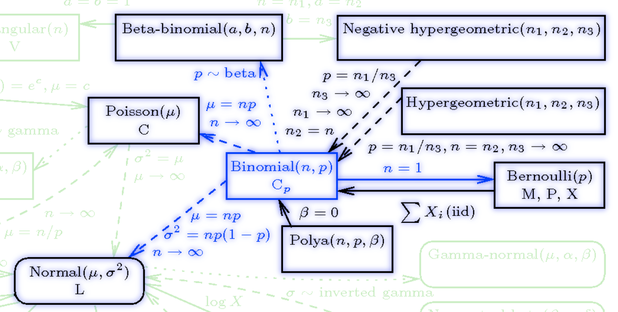{#fig-dbinomial .column-margin width="53mm" group="slides"}
The Binomial Distribution is related to:
- the **Geometric distribution**,
- The **Multinomial distribution** \index{distribution!multinomial} with two categories is the binomial.
- the **Poisson distribution** \index{distribution!Poisson} distribution. If $X \sim \mathrm{Binomial}(n, p)$ rv and $Y \sim \mathrm{Poisson}(np)$ distribution then $\mathbb{P}r(X = n) \approx \mathbb{P}r(Y = n)$ for large $n$ and small $np$.
- the **Bernoulli distribution** If $X \sim \mathrm{Binomial}(n, p)$ RV with $n = 1$, $X \sim Bernoulli(p)$ RV.
- the **Normal distribution** If $X \sim \mathrm{Binomial}(n, p)$ RV and $Y \sim Normal(\mu=np,\sigma=n\mathbb{P}r(1-p))$ then for integers j and k, $\mathbb{P}r(j \le X \le k) \approx \mathbb{P}r(j – {1 \over 2} \le Y \le k + {1 \over 2})$. The approximation is better when $p ≈ 0.5$ and when n is large. For more information, see normal approximation to binomial
- **Hypergeometric**: The difference between a binomial distribution and a hypergeometric distribution is the difference between sampling with replacement and sampling without replacement. As the population size increases relative to the sample size, the difference becomes negligible. So If $X \sim Binomial(n, p)$ RV and $Y \sim HyperGeometric(N,a,b)$ then
$$
\lim_{n\to \infty} X = Y
$$
```{python}
#| label: "binomial-distribution"
import numpy as np
from scipy.stats import binom
import matplotlib.pyplot as plt

fig, ax = plt.subplots(1, 1)
n, p = 5, 0.4
mean, var, skew, kurt = binom.stats(n, p, moments='mvsk')
print(f'{mean=:1.2f}, {var=:1.2f}, {skew=:1.2f}, {kurt=:1.2f}')
x = np.arange(binom.ppf(0.01, n, p), binom.ppf(0.99, n, p))
ax.plot(x, binom.pmf(x, n, p), 'bo', ms=8, label='binom pmf')
ax.vlines(x, 0, binom.pmf(x, n, p), colors='b', lw=5, alpha=0.5)
rv = binom(n, p)
ax.vlines(x, 0, rv.pmf(x), colors='k', linestyles='-', lw=1,
        label='frozen pmf')
ax.legend(loc='best', frameon=False)
plt.show()
## generate random numbers
r = binom.rvs(n, p, size=10)
r
```
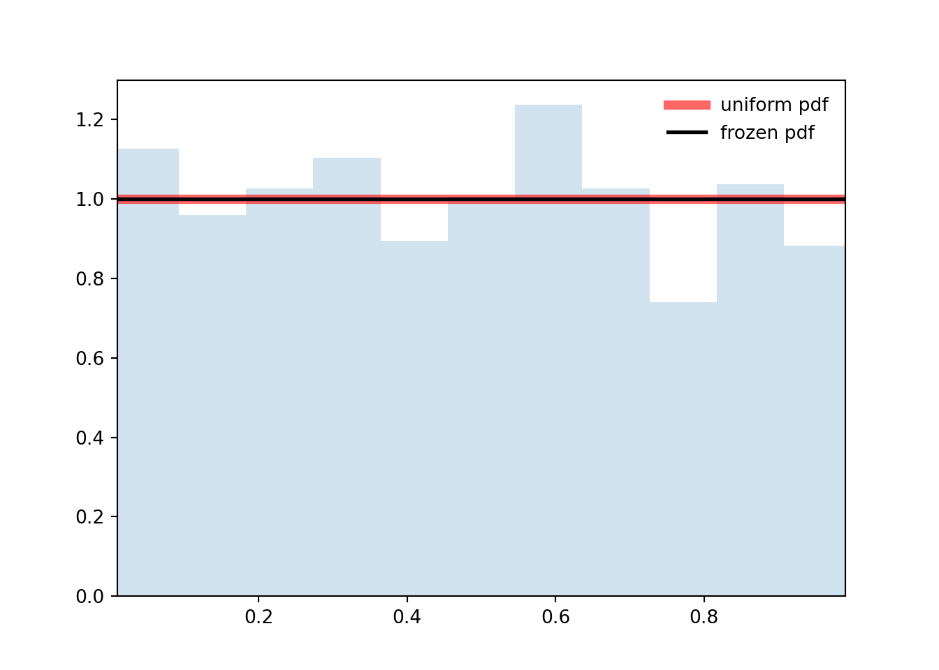
### The Discrete Uniform Distribution
$$
X \sim U[0,1]
$$ {#eq-l3-discrete-uniform-rv}
$$
f(x)=
\begin{cases}
1, & \text{if}\ x \in [0,1] \\
0, & \text{otherwise}
\end{cases}
= \mathbb{I}_{\{0 \le x \le 1\}}(x)
$$ {#eq-l3-uniform-pmf}
```{python}
#| label: "uniform-distribution"
import numpy as np
from scipy.stats import uniform
import matplotlib.pyplot as plt
fig, ax = plt.subplots(1, 1)

n, p = 5, 0.4
mean, var, skew, kurt = uniform.stats(moments='mvsk')
print(f'{mean=:1.2f}, {var=:1.2f}, {skew=:1.2f}, {kurt=:1.2f}')
# we use ppf to get the domain from a range of (0.01,0.99)
x = np.linspace(uniform.ppf(0.01), uniform.ppf(0.99), 100)
ax.plot(x, uniform.pdf(x), 'r-', lw=5, alpha=0.6, label='uniform pdf')
rv = uniform()
ax.plot(x, rv.pdf(x), 'k-', lw=2, label='frozen pdf')

## generate random numbers
r = uniform.rvs(size=1000)

# And compare the histogram:
ax.hist(r, density=True, bins='auto', histtype='stepfilled', alpha=0.2)
ax.set_xlim([x[0], x[-1]])
ax.legend(loc='best', frameon=False)
plt.show()
```
### The Continuous Uniform Distribution
$$
X \sim \mathrm{Uniform}[\theta_1,\theta_2]
$$ {#eq-l3-uniform-rv}
$$
f(x)= \frac{1}{\theta_2-\theta_1} \mathbb{I}_{\{\theta_1 \le x \le \theta_2\}}(x)
$$ {#eq-l3-uniform-pdf}
## The Normal, Z, t Distributions {#sec-the-normal-z-t-distributions}
\index{distribution!normal}
The *normal*, AKA *Gaussian distribution* is one of the most important distributions in statistics.
It arises as the limiting distribution of sums (and averages) of random variables. This is due to the @sec-cl-theorem. Because of this property, the normal distribution is often used to model the "errors," or unexplained variations of individual observations in regression models.
### The Standard Normal distribution {#sec-the-standard-normal-distribution}
\index{distribution!standard normal}
The standard normal distribution is given by
$$
\mathcal{Z} \sim \mathcal{N}[1,0]
$$ {#eq-l3-z-rv}
$$
f(z) = \frac{1}{\sqrt{2 \pi}} e^{-\frac{z^2}{2}}
$$ {#eq-l3-z-pdf}
$$
\mathbb{E}[\mathcal{Z}] = 0
$$ {#eq-l3-z-expectation}
$$
\mathbb{V}ar[\mathcal{Z}]= 1
$$ {#eq-l3-z-variance}
### The Normal distribution
\index{distribution!normal}
Now consider $X = \sigma \mathcal{Z}+\mu$ where $\sigma > 0$ and $\mu$ is any real constant.
Then $\mathbb{E}(X) = \mathbb{E}(\sigma \mathcal{Z}+\mu) = \sigma \mathbb{E}(\mathcal{Z}) + \mu = \sigma \times 0 + \mu = \mu$ and $Var(X) = Var(\sigma^2 + \mu) = \sigma^2 Var(\mathcal{Z}) + 0 = \sigma^2 \cdot 1 = \sigma^2$
Then, X follows a normal distribution with mean $\mu$ and variance $\sigma^2$ (standard deviation $\sigma$) denoted as
$$
X \sim \mathcal{N}[\mu,\sigma^2]
$$ {#eq-l3-normal-rv}
$$
f(x\mid \mu,\sigma^2) = \frac{1}{\sqrt{2 \pi \sigma^2}} e^{-\frac{1}{\sqrt{2 \pi \sigma^2}}(x-\mu)^2}
$$ {#eq-l3-normal-pdf}
$$
\mathbb{E}[x]= \mu
$$ {#eq-l3-normal-expectation}
$$
\mathbb{V}ar[x]= \sigma^2
$$ {#eq-l3-normal-variance}
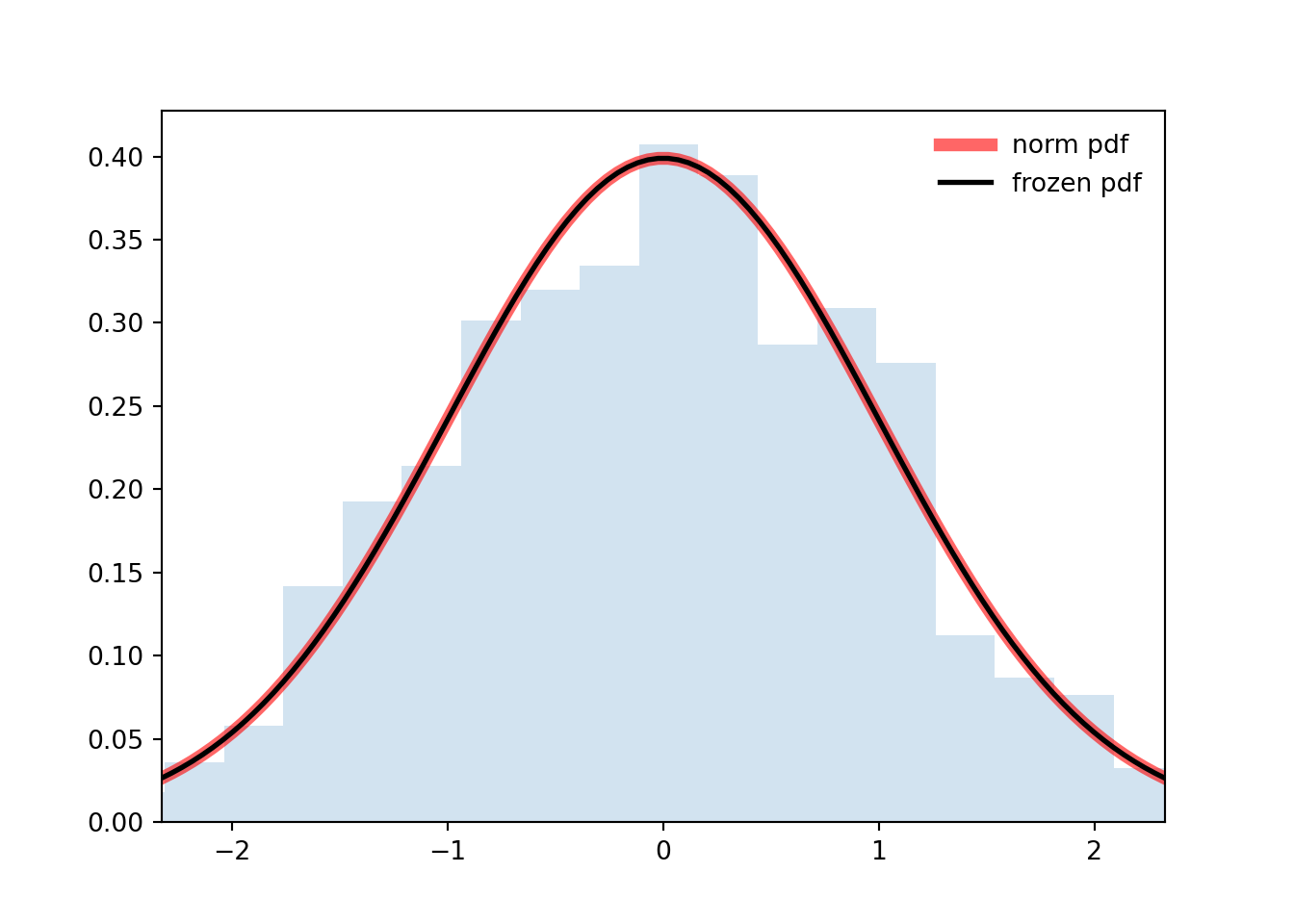
- The normal distribution is symmetric about the mean $\mu$ and is often described as a `bell-shaped` curve.
- Although X can take on any real value (positive or negative), more than 99% of the probability mass is concentrated within three standard deviations of the mean.
The normal distribution has several desirable properties.
One is that if $X_1 \sim \mathcal{N}(\mu_1, \sigma^2_1)$ and $X_2 \sim \mathcal{N}(\mu_2, \sigma^2_2)$ are independent, then $X_1+X_2 \sim \mathcal{N}(\mu_1+\mu_2, \sigma^2_1+\sigma^2_2)$.
Consequently, if we take the average of n Independent and Identically Distributed (IID) normal random variables we have
$$
\bar X = \frac{1}{n}\sum_{i=1}^n X_i \sim \mathcal{N}(\mu, \frac{\sigma^2}{n})
$$ {#eq-l3-normal-sum}
```{python}
#| label: "normal-distribution"
import numpy as np
from scipy.stats import norm
import matplotlib.pyplot as plt
fig, ax = plt.subplots(1, 1)

n, p = 5, 0.4
mean, var, skew, kurt = norm.stats(moments='mvsk')
print(f'{mean=:1.2f}, {var=:1.2f}, {skew=:1.2f}, {kurt=:1.2f}')
x = np.linspace(norm.ppf(0.01),
                norm.ppf(0.99), 100)
ax.plot(x, norm.pdf(x),
       'r-', lw=5, alpha=0.6, label='norm pdf')

rv = norm()
ax.plot(x, rv.pdf(x), 'k-', lw=2, label='frozen pdf')
r = norm.rvs(size=1000)

ax.hist(r, density=True, bins='auto', histtype='stepfilled', alpha=0.2)
ax.set_xlim([x[0], x[-1]])
ax.legend(loc='best', frameon=False)
plt.show()
```
### The t-Distribution
\index{distribution,t}
If we have normal data, we can use (@eq-normal-sum) to help us estimate the mean $\mu$. Reversing the transformation from the previous section, we get
$$
\frac {\hat X - \mu}{\sigma / \sqrt(n)} \sim N(0, 1)
$$ {#eq-l3-t-transform}
However, we may not know the value of $\sigma$. If we estimate it from data, we can replace it with $S = \sqrt{\sum_i \frac{(X_i-\hat X)^2}{n-1}}$, the sample standard deviation. This causes the expression (@eq-t-transform) to no longer be distributed as a Standard Normal; but as a standard *t-distribution* with $ν = n − 1$ `degrees of freedom`
$$
X \sim t[\nu]
$$ {#eq-l3-t-rv}
$$
f(t\mid\nu) = \frac{\Gamma(\frac{\nu+1}{2})}{\Gamma(\frac{\nu}{2})\sqrt{\nu\pi}}\left (1 + \frac{t^2}{\nu}\right)^{-(\frac{\nu+1}{2})}\mathbb{I}_{t\in\mathbb{R}} \qquad \text{(PDF)}
$$ {#eq-l3-t-pdf-gamma}
$$
\text{where }\Gamma(w)=\int_{0}^{\infty}t^{w-1}e^{-t}\mathrm{d}t \text{ is the gamma function}
$$
$$
f(t\mid\nu)={\frac {1}{{\sqrt {\nu }}\,\mathrm {B} ({\frac {1}{2}},{\frac {\nu }{2}})}}\left(1+{\frac {t^{2}}{\nu }}\right)^{-(\nu +1)/2}\mathbb{I}_{t\in\mathbb{R}} \qquad \text{(PDF)}
$$ {#eq-l3-t-pdf-beta}
$$
\text{where } B(u,v)=\int_{0}^{1}t^{u-1}(1-t)^{v-1}\mathrm{d}t \text{ is the beta function}
$$
$$
\mathbb{E}[Y] = 0 \qquad \text{ if } \nu > 1
$$ {#eq-l3-t-expectation-xyz}
$$
\mathbb{V}ar[Y] = \frac{\nu}{\nu - 2} \qquad \text{ if } \nu > 2
$$ {#eq-l3-t-variance}
The t distribution is symmetric and resembles the Normal Distribution but with thicker tails. As the degrees of freedom increase, the t distribution looks more and more like the standard normal distribution.
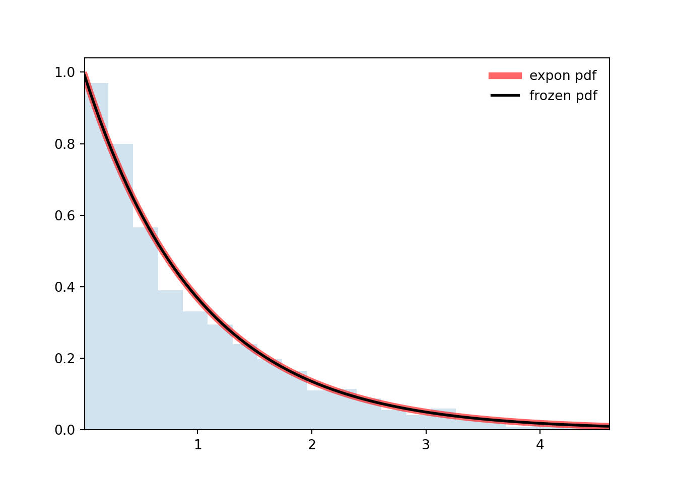
## The Exponential Distribution
\index{Exponential distribution}
The **Exponential distribution** models the waiting time between events for events with a rate $\lambda$. Those events, typically, come from a **Poisson** process.
The **Exponential distribution** is often used to model the `waiting time between random events`. Indeed, if the waiting times between successive events are independent then they form an $\exp(r(\lambda)$ distribution. Then for any fixed time window of length t, the number of events occurring in that window will follow a `Poisson distribution` with mean $t\lambda$.
$$
X \sim Exp[\lambda]
$$ {#eq-l3-exponential-rv}
$$
f(x \mid \lambda) = \frac{1}{\lambda} e^{- \frac{x}{\lambda}}(x)\mathbb{I}_{\lambda\in\mathbb{R}^+ } \mathbb{I}_{x\in\mathbb{R}^+_0 } \quad \text{(PDF)}
$$ {#eq-l3-exponential-pdf}
$$
\mathbb{E}(x)= \lambda
$$ {#eq-l3-exponential-expectation}
$$
\mathbb{V}ar[X]= \lambda^2
$$ {#eq-l3-exponential-variance}
```{python}
#| label: "exponential-distribution"
import numpy as np
from scipy.stats import expon
import matplotlib.pyplot as plt
fig, ax = plt.subplots(1, 1)

n, p = 5, 0.4
mean, var, skew, kurt = expon.stats(moments='mvsk')
print(f'{mean=:1.2f}, {var=:1.2f}, {skew=:1.2f}, {kurt=:1.2f}')
x = np.linspace(expon.ppf(0.01), expon.ppf(0.99), 100)
ax.plot(x, expon.pdf(x), 'r-', lw=5, alpha=0.6, label='expon pdf')

rv = expon()
ax.plot(x, rv.pdf(x), 'k-', lw=2, label='frozen pdf')

r = expon.rvs(size=1000)

ax.hist(r, density=True, bins='auto', histtype='stepfilled', alpha=0.2)
ax.set_xlim([x[0], x[-1]])
ax.legend(loc='best', frameon=False)
plt.show()
```
# Additional Discrete Distributions
## The Geometric Distribution {#sec-the-geometric-distribution}
\index{distribution!geometric}
The **Geometric distribution** arises when we want to know "What is the number of Bernoulli trials required to get the first success?", i.e., the number of Bernoulli events until a success is observed, such as the probability of getting the first head when flipping a coin. It takes values on the positive integers starting with one (since at least one trial is needed to observe a success).
$$
X \sim \mathrm{Geo}(p)
$$ {#eq-l3-geom-rv}
$$
\mathbb{P}r(X = x\mid p) = \mathbb{P}r(1-p)^{x-1} \qquad \forall x \in N;\quad 0\le p \le 1
$$ {#eq-l3-geom-pmf}
$$
\mathbb{E}[X] = \frac{1}{p}
$$ {#eq-l3-geom-expectation}
$$
\mathbb{V}ar[X]=\frac{1-p}{p^2}
$$ {#eq-l3-geom-variance}
$$
\mathbb{M}_X[t] = \frac{pe^t}{1-(1-p)e^t} \qquad t < -log(1-p)
$$ {#eq-l3-geom-mgf}
## The Multinomial Distribution {#sec-the-multinomial-distribution}
\index{distribution!multinomial}
\index{distribution!Bernoulli}
Another generalization of the Bernoulli distribution and the Binomial distribution is the **Multinomial distribution**, which sums the successes of Bernoulli trials when there are n different possible outcomes. Suppose we have n trials and there are k different possible outcomes that occur with probabilities $p_1, \ldots, p_k$. For example, we are rolling a six-sided die that might be loaded so that the sides are not equally likely, then n is the total number of rolls, $k = 6$, $p_1$ is the probability of rolling a one, and we denote by $x_1, \ldots, x_6$ a possible outcome for the number of times we observe rolls of each of one through six, where
$$
X \sim \mathrm{Multinomial}(p_1,...p_k)
$$
$$
P (X = x \mid p_1,\ldots,p_k) = \frac{n!}{x_1! \cdot \cdot \cdot x_k! } \prod_i p_i^{x_i}
$$
## The Poisson Distribution {#sec-the-poisson-distribution}
The **Poisson distribution** \index{distribution!Poisson} arises when modeling **count** data. The parameter $\lambda > 0$ is the `rate` at which we expect to observe the thing we are counting. We write this as $X \sim \mathrm{Poisson}(\lambda)$
$$
\mathbb{P}r(X = x \mid \lambda) = \frac{\lambda^x e^{−\lambda}}{x!} \qquad \forall x \in \mathbb{N}_0 \qquad \text{PDF}
$$ {#eq-l3-poisson-PMF}
$$
\mathbb{E}[X] = \lambda \qquad \text{Expectation}
$$ {#eq-l3-poisson-expectation}
$$
\mathbb{V}ar[X] = \lambda \qquad \text{Variance}
$$ {#eq-l3-poisson-variance}
$$
\mathbb{M}_X(t) = \exp[\lambda(e^t-1)] \qquad \text{Moment Generating fn.}
$$ {#eq-l3-poisson-mgf}
$$
\mathcal{I}_X(t) = \frac{1}{\lambda}
$$ {#eq-l3-poisson-fisher-information}
### Relations
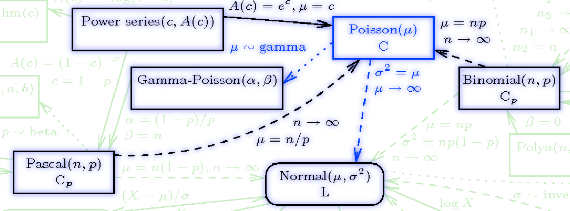{#fig-dPoisson .column-margin width="53mm" group="slides"}
\index{process!Poisson}
A *Poisson process* is a process wherein events occur on average at rate $\mathbb{E}$, events occur one at a time, and events occur independently of each other.
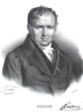{#fig-bio-Poisson .column-margin width="53mm" group="slides"}
::: {.callout-tip}
### Biographical Note on The Siméon Denis Poisson
The Poisson distribution is due to Baron Siméon Denis Poisson (1781-1840) see [@poisson2019english pp. 205-207] was a French mathematician and physicist who worked on statistics, complex analysis, partial differential equations, the calculus of variations, analytical mechanics, electricity and magnetism, thermodynamics, elasticity, and fluid mechanics.
for a fuller [biography see](https://mathshistory.st-andrews.ac.uk/Biographies/Poisson/)
:::
## Hypergeometric Distribution
\index{distribution!hypergeometric}
Consider an urn with $a$ white balls and $b$ black balls. Draw $N$ balls from this urn without replacement. The number white balls drawn, $n$ is Hypergeometrically distributed.
$$
X \sim \mathrm{Hypergeometric}(n \mid N,a,b)
$$
$$
\mathrm{Hypergeometric}(n\mid N,a,b) = \frac{\normalsize{\binom{a}{n} \binom{b}{N - n}}} {\normalsize{\binom{a + b}{N}}} \quad \text{(PDF)}
$$ {#eq-l3-Hypergeometric-pdf}
$$
\mathbb{E}[X]=N\frac{a}{a+b} \qquad \text{(expectation)}
$$ {#eq-l3-Hypergeometric-expectation}
$$
\mathbb{V}ar[X]=N\,\frac{ab}{(a + b)^2}\,\frac{a+b-N}{a+b-1} \qquad \text{(variance)}
$$ {#eq-l3-Hypergeometric-variance}