The following material is based on the Nonparametric Bayes Tutorial that took place in the 2016 ML the University of Cádiz in Cádiz, Spain. Which focuses primarily on the Dirichlet Process and related processes. There is so much material on BNP and non-parametric methods out there it is hard to get started. The speaker has a blog with more material on this and other topics.
I find that MIT Tenured Professor, Tamara Broderick’s explanations are very clear and accessible. She uses simple motivating examples, she shares the basis of how she has built her intuition for the topic. Most significantly she is very enthusiastic about the BNP which I find inspiring and contagious.
I found the videos hard to follow at times, as she is talking fast (a good thing). So I watched them a number of times at my leisure. Many times I found myself surprised by things she said. But each time I checked I not only learned something new but was able to put aside some of my misconceptions.
I want to develop the generative and behavioral stories that help us connect the abstract stochastic processes to problems we might want to solve in the real world. Again this is something I have already stated on in earlier notes in course 1 and the appendices on distributions.
114.1 Nonparametric Bayes
- Bayesian Nonparametrics (BNP) = Bayesian + Nonparametric
- The Bayesian part should be familiar to us at this point. Here is how we fuse data and beliefs during an experiment:
\underbrace{\mathbb{P}r(parameters \mid data)}_{\substack{\text{our beliefs about the params.} \\ \text{at the end of the experiment}}} \propto \underbrace{\mathbb{P}r(data \mid parameters)}_{\substack{\text{data we collected} \\ \text{in our experiment}}} \underbrace{\mathbb{P}r(parameters)}_{\substack{\text{prior beliefs about params.} \\ \text{going into our experiment}}} \qquad \tag{114.1}
- Non-parametric is a bit of a misnomer, it does not mean we don’t have parameters but rather that we reduce our restrictions on parameters like:
- from independence and identically distributed items to exchangeable1, and
- from fixed and finite to a growing and unbounded i.e. a potentially infinite family of parameters
This empowers us to model more complex data and phenomena there complexity grows as data accrues.
- Some Examples:
- Topic modeling for Wikipedia articles
- Classifying/Clustering Species (Jin, He, and Zhang 2012) c.f. DNA Bar coding Reveals Diversity of Parasitoid Wasps in Great Smoky Mountains
- Density Estimation (Escobar and West 1995) (Ghosal, Ghosh, and Ramamoorthi 1999)
- Survival analysis curves
- Fitness exercises (K. C. R. Fox et al. 2014)
- Genetics (Ewens 1972), (Hartl and Clark 2006)
- Health issues in newborn babies (Saria et al. 2010)
- Social networks (Lloyd et al. 2012) (Miller, Jordan, and Griffiths 2009)
- Images (Sudderth and Jordan 2008)
- Time series (E. Fox et al. 2011), (E. Fox et al. 2009)
114.2 Nonparametric Bayes
Next The speaker is vehemently excited about de Finetti’s theorem. This is a key theoretical motivation for BNP. And without the BNP the theorem is not that interesting or as easy to understand.
- A theoretical motivation: De Finetti’s Theorem
- A data sequence is infinitely exchangeable if the distribution of any N data points doesn’t change when permuted
- This is a much weaker assumption than independence and Exchangeability is the prerequisite for De Finetti’s theorem:
p(X_1, \ldots , X_N ) = p(X_{\sigma(1)} , \ldots , X_{\sigma(N)} ) \tag{114.2}
De Finetti’s Theorem (roughly): A sequence is infinitely exchangeable \iff, for all N and some distribution P over parameters \theta, p(X_1, \ldots , X_N ) = \int_\theta \prod_{}^N p(X_n\mid\theta)P(d\theta)
Motivates:
- Parameters and likelihoods
- Priors
- “Nonparametric Bayesian” priors
Note: that De Finetti’s proved his theorem in 1931 but for finite exchangeable sequences.
In (Hewitt and Savage 1955) Leonard J. Savage and Edwin Hewitt extended the result from finite to infinite exchangeability in 1955.
In (Diaconis and Freedman 1980) Persi Diaconis and David Freedman in the 1970s extended the result to Markov chains. These bake in the Markov property but it is not as strong as IID.
- TODO: try for a review of this paper
In (Aldous 1983) David Aldous proved a more general for arrays 1983.
- TODO: try for a review of this paper.
I think this is the most mathematically advanced slide in the tutorial.
First let me point out that this is however a result we already covered in course 1 but as I just explained de Finetti only covered the finite case which is all we needed so far.
For Hierarchical models I.I.D. is a strong assumption but we can often fall back to assume exchangeability.
For time series models I.I.D. is too strong an assumption but exchangeability is often reasonable.
For BNP we would need to use the stronger forms of the theorem by Aldous. (I haven’t yet found the citations for the work by Diaconis and Freedman. But Diaconis wrote extensively on exchangeability in the context of Combinatorics and Markov Chains which Aldous also worked on.)
three final thought on the theorem:
- The BNP problem settings lets us not only use the general theorem but also provides problems that motivate it.
- I find myself wondering if de Finetti shows us that exchangeability implies a conditional independence structure than what does he mean by insisting that “Probability does not exist” (his famous dictum). The theorem seems to be a machine taking weak subjective assumptions on the events and turning them into a strong objective structure.
- In deep learning the most powerful models are sequence models (LSTMs, transformers and state space approaches) and one might be able to put consider all these into an abstract framework using BNP and De Finetti’s theorem and exchangeability.
- TODO: check if Herbert Lee did something this in his book.
114.3 The Dirichlet Process
114.3.1 Background
- We want to develop an intuition for the Dirichlet Process (DP).
- According to the speaker, the DP can be viewed as the archtype of BNP models.
- Once you mastered the DP you can understand papers in this field and most other BNP models. She uses the analogy of mastering your first programming language and then you can learn other languages far more easily.
- We usually use it together with some likelihood function to build a nonparametric model.
- Once we understand the DP we look at the closely related Chinese Restaurant Process (CRP) and the stick-breaking construction. We should then understand how these three relate to each other. (Why do we want these different processes?)
- Finally the tutorial will cover what other nonparametric processes exist and when to use them. (And I will consider if they deserve a full lectures in this course notes.)
114.3.2 Generative Model
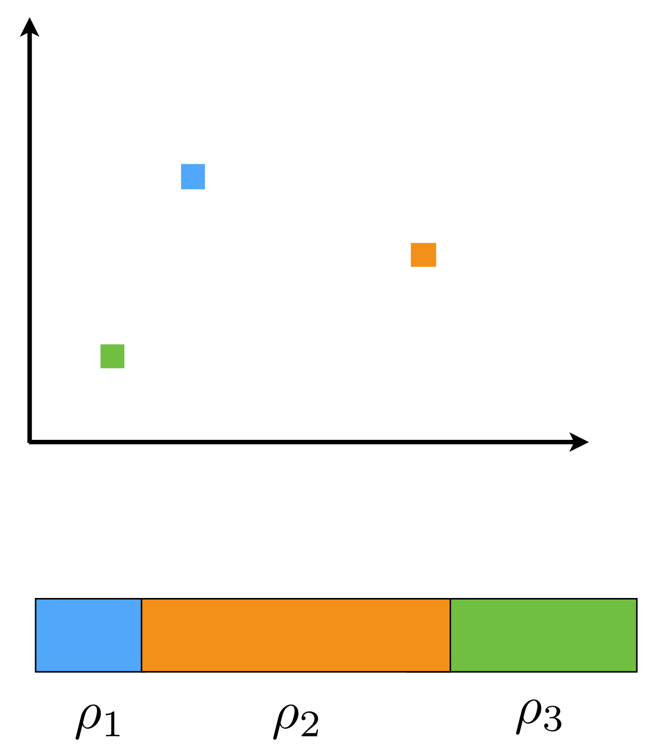
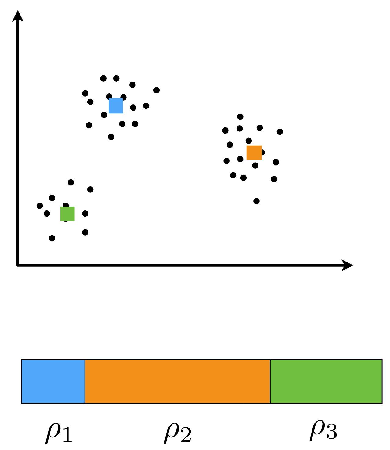
The DP is often used with another likelihood function to build a nonparametric model. In this case we will use it with a Finite Gaussian Mixture to build a clustering model for a set of points.
Recall our material for mixture models: we have k=2 components in our mixture and one way we can set things up is to generate a component selector z_n for each data point then to use it to draw the data point x_n from the normal distribution associated with the selected component.
114.3.2.1 The Generative model as a Story:
Lets start a story:
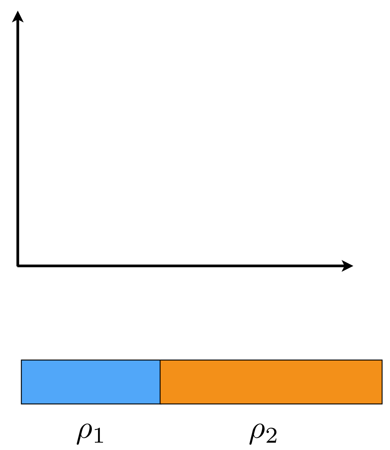
- Finite Gaussian mixture model (K=2 clusters)
- We start by generating a component selector z_n from two clusters by drawing it from a Categorical distribution with parameters \rho_1 and \rho_2. In this case these parameters are simply the probabilities of selecting each of the two clusters and since we have two clusters \rho_2 = 1 - \rho_1.
- However, we do not know these parameters, so we will be putting a prior on them.
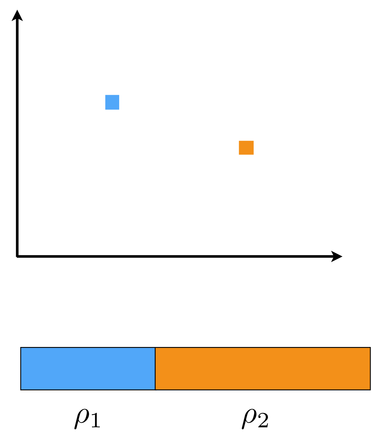
- Next we generate the data points x_n from a normal distribution with mean \mu_0 and covariance \Sigma. We assume that the data points are independent given the cluster assignments.
- Again we don’t know the means of the clusters so we will put a prior on them as well.
Actually this is a bit backwards, thinking causally we need to start at the top of the PGM plate model ((priors or hyper-priors) and work our way down.
So at the end of the slide the instructor summarizes the generative story as follows:
- we generate the weights \rho_1, \rho_2 for the two clusters from a Beta distribution with parameters \alpha_0, \beta_0.
- we generate the means \mu_1, \mu_2 for the two clusters from a normal distribution with mean \mu_0 and variance \sigma_0^2.
- we generate the points x_n from a normal distribution with mean \mu_{z_n} and covariance \Sigma where z_n is the cluster assignment for point n.
114.3.2.2 The Hierarchical Model for the Generative Story:
we can write this as follows: \begin{aligned} z_n & \stackrel{iid}{\sim} \text{Categorical}(\rho_1, \rho_2) && \text{cluster assignments} \\ x_n & \stackrel{indep}{\sim} \mathcal{N}(\mu_0, \Sigma) && \text{data points} \\ \rho_1 & \sim \text{Beta}(\alpha_0, \beta_0) && \text{prior for weights} \\ \rho_2 & = 1 - \rho_1 && \text{since } K=2 \\ \mu_k & \stackrel{iid}{\sim} \mathcal{N}(\mu_0, \sigma_0^2), \quad k=1,2 && \text{prior for means} \end{aligned} \tag{114.3}
We do not know \mu_1 , \mu_2, \rho_1 , \rho_2
We assume the quantities \Sigma, \sigma_0^2, \mu_0, \alpha_0, \beta_0 are fixed and known to keep things simple but the instructor notes that we we could also put priors on these hyperparameters.
Inference goal: assignments of data points to clusters, cluster parameters. \mathbb{P}r(parameters \mid data) \propto \mathbb{P}r(data \mid parameters)\; \mathbb{P}r(parameters)
114.3.3 The Beta Distribution (review)
We just used the Beta distribution in our generative model for a two component Gaussian mixture.
- We picked the Beta distribution for a number of reasons:
- We said that it a good choice for a prior because it is the conjugate prior for the Categorical distribution.
- I found that odd as I recall that the Dirichlet distribution is the conjugate prior for the Binomial, bernoulli, negative binomial and geometric distributions but not the Categorical distribution.
- What about the Categorical distribution how did we miss that one? I was stumped except that when K=2 the Categorical distribution is equivalent to the Bernoulli distribution. 🤥 And when K gets bigger we will need to use a Dirichlet prior and the categorical will be a non-degenerate case which no longer a Bernoulli distribution. However we are building up to the case where K is unbounded. So even if it is a but of a stretch this is actually a clever point that the instructor is making. 🤭
- The Beta distribution is a distribution over the interval [0,1] which is a good choice when we want to draw a probabilities. And we are setting the prior for the probabilities of selecting each cluster.
- The Beta distribution is more flexible than the Binomial as it can if we want it to be a uniform distribution! This is where it Beta trumps the Binomial!
- If we have a good understanding of the Binomial distribution we can use it to build an intuition for most discrete cases for the Beta distribution.
- We said that it a good choice for a prior because it is the conjugate prior for the Categorical distribution.
It turns out that the Categorical distribution is a special case of the Multinomial distribution. And the Dirichlet distribution is the conjugate prior for the Multinomial distribution.
It certainly looks like the Bernoulli distribution once you understand that the Gamma functions are just Binomial coefficients. And if we look at the non gamma part it looks like the likelihood of a Bernoulli distribution. I.e. it seems like we are summing all the ways one can get a certain number of successes and failures in a series of Bernoulli trials.
It turns out that the Beta distribution is a special case of the Dirichlet distribution. We need to understand it well, as we can use it in a number of constructions of the Dirichlet Process. Once we have a basic intuition for the Beta distribution we can extend it to the Dirichlet distribution and then to the Dirichlet Process. So let us review it.
The Beta distribution is a distribution over the interval [0,1]. It is often used as a prior for probabilities. It is the conjugate prior for the Categorical distribution.
\text{Beta}(\rho \mid \alpha_1, \alpha_2) = \frac{\Gamma(\alpha_1 + \alpha_2)}{\Gamma(\alpha_1)\Gamma(\alpha_2)} \rho^{\alpha_1 - 1} (1 - \rho)^{\alpha_2 - 1}
\alpha_1, \alpha_2 > 0
\rho \in [0,1]
A few point here first about the Gamma function \Gamma
- integer m: \Gamma(m+1) = m!
- for x > 0: \Gamma(x+1) = x\Gamma(x)
Now the instructor points out correctly that these Gamma functions are just Binomial coefficients when we are dealing with integers. In
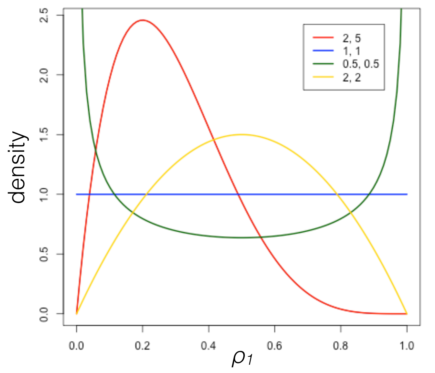
-Now let’s look at the shape of the Beta distribution for different values of \alpha_1 and \alpha_2. - What happens? - 1 = a_1 = a_2 \implies Beta(1,1)=\frac{1!}{0! \times 0!}\rho^{0}(1-\rho)^{0} = 1
- This is a uniform distribution over regardless of the value of \rho. - a = a_1 = a_2 \to \infty \implies \text{Beta}(a,a) is highly concentrated at around 0.5 and almost zero elsewhere. - a_1 > a_2 \implies \text{Beta}(a_1, a_2) is skewed to the left - a_1 < a_2 \implies \text{Beta}(a_1, a_2) is skewed to the right
- Beta is conjugate to Cat
\rho \sim \text{Beta}(\alpha_1, \alpha_2),\qquad z \sim \text{Cat}(\rho_1, \rho_2)
p(\rho_1 , z) \propto \rho_1^{\mathbb{1}_{z=1}} (1 - \rho_1 )^{\mathbb{1}_{z=2}} \rho_1^{a_1 -1} (1 - \rho_1 )^{a_2 -1}
p(\rho_1 , z) \propto \rho_1^{\mathbb{1}_{z=1-1}} (1 - \rho_1 )^{\mathbb{1}_{z=2}-1} \propto \text{Beta}(\rho_1 \mid a_1 + \mathbb{1}_{z=1}, a_2 + \mathbb{1}_{z=2})
114.3.4 Beta Distribution Playground
#| '!! shinylive warning !!': |
#|   shinylive does not work in self-contained HTML documents.
#|   Please set `embed-resources: false` in your metadata.
#| standalone: true
#| viewerHeight: 420
#| components: [viewer] #editor
from __future__ import annotations

import numpy as np
import pandas as pd
import altair as alt

from shiny import App, reactive, render, ui
from shinywidgets import output_widget, render_altair

# ---- UI ---------------------------------------------------------------------
app_ui = ui.page_fluid(
    ui.layout_sidebar(
        ui.sidebar(
            ui.h3("Parameters"),
            ui.input_slider("a", "a (alpha)", min=0.1, max=100.0, value=2.0, step=0.1),
            ui.input_slider("b", "b (beta)", min=0.1, max=100.0, value=2.0, step=0.1),
            ui.input_action_button("draw", "Draw", class_="btn-primary"),
            ui.input_action_button("reset", "Reset"),
        ),
        ui.layout_columns(
            ui.card(
                ui.card_header("Latest draw: probabilities over {1, 2}"),
                output_widget("w_bar"),
                ui.output_text("latest_label"),
            ),
            ui.card(
                ui.card_header("Histogram of draws ρ"),
                output_widget("w_hist"),
                ui.output_text("count_label"),
            ),
        )
    ),
    title="Beta(a, b) — ShinyLive Demo"
)

# ---- Server -----------------------------------------------------------------

def server(input, output, session):
    samples = reactive.Value(np.array([], dtype=float))

    @reactive.effect
    @reactive.event(input.reset)
    def _reset():
        samples.set(np.array([], dtype=float))

    @reactive.effect
    @reactive.event(input.draw)
    def _draw_one():
        a = float(input.a())
        b = float(input.b())
        rho = float(np.random.beta(a, b))
        xs = samples()
        samples.set(np.concatenate([xs, [rho]]))

    @render.text
    def latest_label():
        xs = samples()
        if xs.size == 0:
            return "No draws yet. Click ‘Draw’."
        rho = float(xs[-1])
        return f"ρ (latest) = {rho:.4f}; 1−ρ = {1 - rho:.4f}"

    @render_altair
    def w_bar():
        xs = samples()
        if xs.size == 0:
            df = pd.DataFrame({"index": ["1", "2"], "prob": [0.0, 0.0]})
        else:
            rho = float(xs[-1])
            df = pd.DataFrame({"index": ["1", "2"], "prob": [rho, 1 - rho]})

        return (
            alt.Chart(df)
            .mark_bar()
            .encode(
                x=alt.X("index:N", title="index"),
                y=alt.Y("prob:Q", scale=alt.Scale(domain=[0, 1]), title="probability"),
                tooltip=[
                    alt.Tooltip("index:N", title="index"),
                    alt.Tooltip("prob:Q", format=".4f", title="probability"),
                ],
            )
            .properties(height=260, title=f"(ρ₁, ρ₂) ~ Beta({input.a():.1f}, {input.b():.1f})")
        )

    @render.text
    def count_label():
        return f"Total draws: {samples().size}"

    @render_altair
    def w_hist():
        xs = samples()
        if xs.size == 0:
            note = pd.DataFrame({"note": ["Click Draw to start"]})
            return alt.Chart(note).mark_text(size=16).encode(text="note:N")

        df = pd.DataFrame({"rho": xs})
        return (
            alt.Chart(df)
            .mark_bar()
            .encode(
                x=alt.X("rho:Q", bin=alt.Bin(maxbins=30), title="ρ"),
                y=alt.Y("count():Q", title="count"),
                tooltip=[alt.Tooltip("count():Q", title="count")],
            )
            .properties(height=300)
        )

app = App(app_ui, server)
114.4 N-component gaussian mixture model
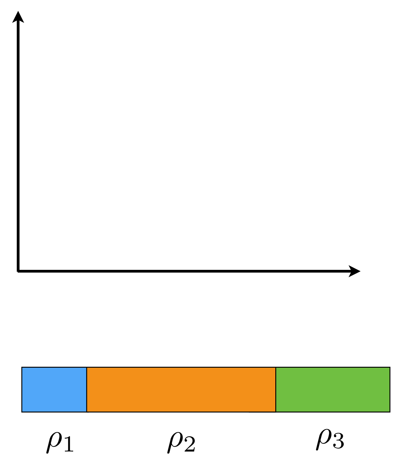
we now move to the case where we have K components in our mixture model
114.4.1 Generative story for K components
summarizes the generative story as follows:
- we draw the weights $_{1:k}, $ for the each cluster from a Dirichlet distribution with parameters \alpha_{0:K}.
- we generate the means \mu_1, \mu_2 for the two clusters from a normal distribution with mean \mu_0 and variance \sigma_0^2.
- we generate the points x_n from a normal distribution with mean \mu_{z_n} and covariance \Sigma where z_n is the cluster assignment for point n.
114.4.1.1 The Hierarchical Model for the Generative Story:
\begin{aligned} \rho_{1:K} & \sim \text{Dirichlet}(\alpha_{1:k}) && \text{cluster weights} \\ \mu_k & \stackrel{iid}{\sim} \mathcal{N}(\mu_0, \sigma_0^2), \quad k=1,2 && \text{cluster means} \\ z_n & \stackrel{iid}{\sim} \text{Categorical}(\rho_{1:k} && \text{point cluster assignments} \\ x_n & \stackrel{indep}{\sim} \mathcal{N}(\mu_0, \Sigma) && \text{point generation} \\ \end{aligned} \tag{114.4}
114.5 Dirichlet distribution Review
Although we have looked at the Dirichlet distribution in the context of Bayesian Mixture Models we will now dive deeper into this distribution and its properties.
BNPs teach us that the Dirichlet distribution is a conjugate prior for the categorical distribution. And to a large extent is the basic building block of non-parametric Bayesian methods.
Once you understand the Dirichlet distribution, you should be able to understand 50% of the non-parametric Bayesian methods used in research today. I found that this lesson does for me what early differential equations did for me in my undergraduate studies. It is a key concept that opens the door to understanding many other concepts. We will see that the Dirichlet distribution is a generalization of the Beta distribution and that it is also a stepping stone to the Chinese Restaurant Process.
We start with the Dirichlet distribution, which is a distribution over a simplex. A simplex is a generalization of a triangle to higher dimensions. For example, in 2D, a simplex is a triangle, and in 3D, it is a tetrahedron. Why a simplex? Because we want to model probabilities, and probabilities must sum to 1. A simplex is a set of points that satisfy this constraint.
Here is the pdf for the Dirichlet distribution:
\text{Dirichlet}(\rho \mid \alpha_1, \ldots , \alpha_K) = \frac{\Gamma(\sum_{k=1}^K \alpha_k)}{\prod_{k=1}^K \Gamma(\alpha_k)} \prod_{k=1}^K \rho_k^{\alpha_k - 1} \qquad a_k>0 \tag{114.5}
- where \rho_k is the k-th component of the vector \rho and
- \alpha_k is the concentration parameter for the k-th component.
- \Gamma is the gamma function, which is a generalization of the factorial function. Recall that \Gamma(n) = (n-1)! for positive integers n.
The concentration parameters control how concentrated the distribution is around the mean.
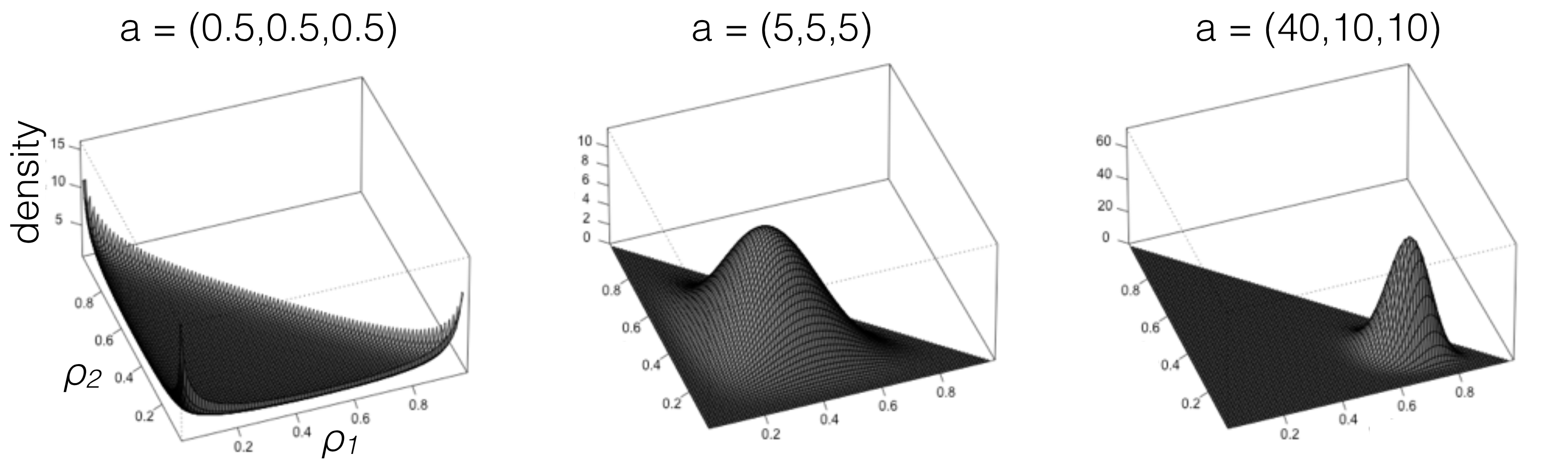
Now we should develop some intuition about the Dirichlet distribution with respect to its parameters.
- what happen when a=a_1=a_K=1?
- what happen when a=a_1=a_K \to 0?
- what happen when a=a_1=a_K \to \infty?
\rho_{1:K} \sim \textrm{Dirichlet}(a_{1:K}) \quad z\sim \textrm{Cat}(\rho_{1:K})
\rho_{1:K}|z \stackrel{d}{=} \textrm{Dirichlet}(a_{1:K}) \quad a'_k= a_k + \mathbb{1}_{\{z=k\}}
- what happen when a_1 > a_2?
114.5.1 Dirichlet Distribution Playground
#| '!! shinylive warning !!': |
#|   shinylive does not work in self-contained HTML documents.
#|   Please set `embed-resources: false` in your metadata.
#| standalone: true
#| viewerHeight: 520
#| components: [ viewer] # editor,

from __future__ import annotations

import numpy as np
import pandas as pd
import altair as alt
from math import sqrt

from shiny import App, reactive, render, ui
from shinywidgets import output_widget, render_altair

# --- Helpers ------------------------------------------------------------------

def dirichlet_sample(a1: float, a2: float, a3: float) -> np.ndarray:
    return np.random.dirichlet(np.array([a1, a2, a3])).astype(float)

def barycentric_to_cartesian(r1: float, r2: float, r3: float) -> tuple[float, float]:
    """
    Map (r1,r2,r3), sum=1, to 2D coords of an equilateral triangle with vertices:
      v1=(0,0) for component 1
      v2=(1,0) for component 2
      v3=(0.5, sqrt(3)/2) for component 3
    """
    x = r2 + 0.5 * r3
    y = (sqrt(3) / 2.0) * r3
    return x, y

def triangle_frame_df() -> pd.DataFrame:
    # outline of triangle for plotting
    verts = [(0.0, 0.0), (1.0, 0.0), (0.5, sqrt(3)/2), (0.0, 0.0)]
    return pd.DataFrame({"x": [v[0] for v in verts], "y": [v[1] for v in verts]})

# --- UI -----------------------------------------------------------------------

app_ui = ui.page_fluid(
    ui.layout_sidebar(
        ui.sidebar(
            ui.h3("Dirichlet(α₁, α₂, α₃)"),
            ui.input_slider("a1", "α₁", min=0.1, max=100.0, value=2.0, step=0.1),
            ui.input_slider("a2", "α₂", min=0.1, max=100.0, value=2.0, step=0.1),
            ui.input_slider("a3", "α₃", min=0.1, max=100.0, value=2.0, step=0.1),
            ui.input_action_button("draw", "Draw", class_="btn-primary"),
            ui.input_action_button("reset", "Reset"),
            ui.hr(),
            ui.output_text("summary_text"),
        ),
        ui.layout_columns(
            ui.card(
                ui.card_header("Latest draw: probabilities over {1, 2, 3}"),
                output_widget("w_bar"),
                ui.output_text("latest_text"),
            ),
            ui.card(
                ui.card_header("All draws on the 2D simplex (ternary)"),
                output_widget("w_ternary"),
                ui.output_text("count_text"),
            ),
        )
    ),
    title="Dirichlet(α₁, α₂, α₃) — ShinyLive Demo"
)

# --- Server -------------------------------------------------------------------

def server(input, output, session):
    # Store draws as an (n, 3) array
    samples = reactive.Value(np.zeros((0, 3), dtype=float))

    @reactive.effect
    @reactive.event(input.reset)
    def _reset():
        samples.set(np.zeros((0, 3), dtype=float))

    @reactive.effect
    @reactive.event(input.draw)
    def _draw_one():
        a1 = float(input.a1())
        a2 = float(input.a2())
        a3 = float(input.a3())
        rho = dirichlet_sample(a1, a2, a3)
        xs = samples()
        samples.set(np.vstack([xs, rho[None, :]]))

    @render.text
    def latest_text():
        xs = samples()
        if xs.shape[0] == 0:
            return "No draws yet. Click ‘Draw’."
        r1, r2, r3 = xs[-1]
        return f"ρ (latest) = ({r1:.4f}, {r2:.4f}, {r3:.4f})"

    @render.text
    def count_text():
        return f"Total draws: {samples().shape[0]}"

    @render.text
    def summary_text():
        a1 = float(input.a1()); a2 = float(input.a2()); a3 = float(input.a3())
        s = a1 + a2 + a3
        mean = (a1/s, a2/s, a3/s)
        # Var for component i: α_i(α₀-α_i) / (α₀²(α₀+1)) for covariances; for scalar var use α_i(α₀-α_i)/(α₀²(α₀+1))
        # Here we just show the mean—clean and informative.
        return f"E[ρ] = ({mean[0]:.4f}, {mean[1]:.4f}, {mean[2]:.4f})"

    @render_altair
    def w_bar():
        xs = samples()
        if xs.shape[0] == 0:
            df = pd.DataFrame({"index": ["1", "2", "3"], "prob": [0.0, 0.0, 0.0]})
        else:
            r1, r2, r3 = xs[-1]
            df = pd.DataFrame({"index": ["1", "2", "3"], "prob": [r1, r2, r3]})

        a1 = float(input.a1()); a2 = float(input.a2()); a3 = float(input.a3())
        return (
            alt.Chart(df)
            .mark_bar()
            .encode(
                x=alt.X("index:N", title="index"),
                y=alt.Y("prob:Q", scale=alt.Scale(domain=[0, 1]), title="probability"),
                tooltip=[
                    alt.Tooltip("index:N", title="index"),
                    alt.Tooltip("prob:Q", format=".4f", title="probability"),
                ],
            )
            .properties(
                width="container",
                height=260,
                title=f"ρ ~ Dirichlet({a1:.1f}, {a2:.1f}, {a3:.1f})",
            )
        )

    @render_altair
    def w_ternary():
        xs = samples()
        tri = triangle_frame_df()

        if xs.shape[0] == 0:
            base = (
                alt.Chart(tri)
                .mark_line()
                .encode(x="x:Q", y="y:Q")
            )
            return (
                base
                .properties(width="container", height=320)
                .configure_axis(grid=False, ticks=False)
            )

        # Map all draws to triangle coords
        cart = np.array([barycentric_to_cartesian(r1, r2, r3) for r1, r2, r3 in xs])
        df_pts = pd.DataFrame({
            "x": cart[:, 0],
            "y": cart[:, 1],
            "r1": xs[:, 0],
            "r2": xs[:, 1],
            "r3": xs[:, 2],
            "idx": np.arange(1, xs.shape[0] + 1),
        })

        base = (
            alt.Chart(tri)
            .mark_line()
            .encode(x="x:Q", y="y:Q")
        )

        pts = (
            alt.Chart(df_pts)
            .mark_circle(opacity=0.6)
            .encode(
                x=alt.X("x:Q", title=None, scale=alt.Scale(domain=[-0.05, 1.05])),
                y=alt.Y("y:Q", title=None, scale=alt.Scale(domain=[-0.05, (sqrt(3)/2)+0.05])),
                tooltip=[
                    alt.Tooltip("idx:Q", title="#"),
                    alt.Tooltip("r1:Q", format=".4f", title="ρ₁"),
                    alt.Tooltip("r2:Q", format=".4f", title="ρ₂"),
                    alt.Tooltip("r3:Q", format=".4f", title="ρ₃"),
                ],
            )
        )

        # Add vertex labels
        lbls = pd.DataFrame({
            "x": [0.0, 1.0, 0.5],
            "y": [0.0, 0.0, sqrt(3)/2],
            "lab": ["1", "2", "3"],
        })
        labels = (
            alt.Chart(lbls)
            .mark_text(dy=-8)
            .encode(x="x:Q", y="y:Q", text="lab:N")
        )

        return (
            (base + pts + labels)
            .properties(width="container", height=320)
            .configure_axis(grid=False, ticks=False, labels=False)
        )

app = App(app_ui, server)- some comments on the code above:
- we need to stretch it so that the plot on the right is triangular
- We have more of a scatter plot than a density plot. It would be better if we could view the density building up as we draw more samples.
- Perhaps adding contours,
- perhaps break it into bins (hexagonal or triangular) and use a heat map.
- Perhaps we can add a z-axis and make it a 3D plot.
114.6 More Classes than points K>N
We have gotten to one of the strongest reasons to use BNP models. When we deal with data we often have more columns than rows. For example, - in genetics we may have a few hundred samples but thousands of genes. - on the web we may have thousands of interactions but billions users, millions of websites and ads. - In text analysis we may have a few hundred documents or sentences but thousands of words. - In image analysis we may have millions of images but potentially infinite number of captions, segmentation.
Yet for almost all ML models assume a fixed K (number of classes, clusters or components). So far we haven’t actually discussed how to handle this but we will in the next section. Before we can do that we will want to highlight a new distinction we have not yet made.
The main point we need to make goes back to an idea we covered in course 3 on mixture models when we discussed density estimation. As I Recall the advantage of mixtures is that they can learn complex densities with a small number of components. The original formulation without mixtures used an array of basis functions (e.g. Gaussians) and then learned the weights for all the basis function. Mixtures go further and let us drop the basis functions that have zero weight. This is what we want to do here but in a more general sense we want to have a number of components that is not fixed (i.e. potentially infinite) but to only have to deal with finite number number of clusters which are the ones that have at least one data point assigned to them. That way we get to handle infinite complexity using finite resources.
To summarize
- Components: the number of latent groups
- CClusters: the number of components represented in the data.
Next we have a couple of demos.
First we look at generating different Dirichlet with 1000 components. We use a innovation parameter alpha and we can see different results.
One setting gives a partition with a few large components and all the others being smaller. My intuition is that they are smaller by orders of magnitude. The second setting gives a more uniform distribution for the components. In fact if we went to an sufficiently large number of components on the way to infinity I think that pretty soon we would get infinitesimal. Components. We may soon be able to test this intuition. But the idea of these demos is to build intuitions about the mechanisms and we will be looking at a number of these next. If we have these handy we may be able to get subtly different behaviors out of this model by using different mechanisms.
In the second demo we consider how quickly clusters are filled as we draw points from a uniform distribution and see which component they belong to.
If we have some large components we soon (after 20 draws) seem to have covered almost all the area in the [0,1] interval with the first few clusters. This is in stark contrast to the fact that there are 1000 components. We now investigate how the growth of the number of clusters as we draw more points for different Dirichlet distribution parametrization.
We again look at two settings and we see the one described above but for a second more uniform partition we see what seems to be a near linear growth in the number of clusters however eventually we see that this pattern is deceptive many more partitions need to be drawn but soon we see that some clusters are being filled more than than others indicating that they are substantially larger. So even with a much more uniform partition there are sufficient fluctuations that a few clusters accumulate for most of the mass. Fundamentally we are observing a power law behavior.
TODO: create an online demo for exploring the dirichlet distribution in greater depth.
Number of clusters for N data points is < K and random
114.7 Choosing K = \infty
Here, difficult to choose finite K in advance (contrast with small K): don’t know K, difficult to infer, streaming data
How to generate K = \infty strictly positive frequencies that sum to one?
- Observation: \rho_{1:K} \sim \text{Dirichlet}((a_{1:K}))
\implies \rho_1 \stackrel{d}{=} Beta(a_1, \sum^K_{k=1}a_k= a_1) \perp \frac{\rho_2,\ldots,\rho_K}{1-\rho_1} \stackrel{d}{=} Dirichlet(a_{2}, \ldots , a_{K} )
“Stick breaking” construction [Sethuraman, 1994]:
\begin{aligned} V_1 &\sim Beta(a_1, a_2 + a_3 + a_4) &&\implies \rho_1 = V_1 \\ V_2 &\sim Beta(a_2, a_3 + a_4) &&\implies \rho_2 = (1 - V_2) V_2 \\ V_3 &\sim Beta(a_3, a_4) &&\implies \rho_3 = (1-V_1)(1 - V_2) V_3 \\ & && \implies \rho_4 = (1-\sum_{k=1}^3 \rho_k) \end{aligned}
- Dirichlet process stick-breaking a_k=1, b_k=\alpha > 0 \begin{aligned} V_1 &\sim Beta(a_1, a_2 + a_3 + a_4) && \rho_1 = V_1 \\ V_2 &\sim Beta(a_2, a_3 + a_4) && \rho_2 = (1 - V_2) V_2 \\ V_k & \sim Beta(a_k,b_k) && \rho_k = \left [ \prod_{k=1}^{k-1} (1-V_j)\right ] V_k \end{aligned}
114.7.1 Bibliographic Review
The instructor provides a number of references for at this point
- (Ferguson 1973) - Ferguson’s paper on the Dirichlet process in which he introduced the random measure and a construction mapping from H to G. This paper lacks details on how to sample from the DP. At this point it was more about the existence and uniqueness proofs for the DP. This is some solid bit of mathematics for when you break new ground and have no foundations to stand on so you dig down to the axioms or near by some properties like conjugacy and the fact that it is a distribution over distributions.
- (blackwell1973PolyaUrn?) - Blackwell and MacQueen’s paper on the Polya urn scheme for sampling from the DP. This paper also introduced the Chinese Restaurant Process
- (Sethuraman 1994) - Sethuraman’s paper on the stick breaking construction of the Dirichlet process.
The other papers seem to be about the GEM and sampling methods.
(McCloskey 1965) - McCloskey Phd Thesis dealing with the problem of enumerating (clustering) species in an ecological context. This is an first paper one the GEM distribution for sampling infinite partitions.
(ENGEN 1975) - Engen’s work dealing with the same problem.
(Patil and Taillie 1982) - not clear why this is cited.
(Ewens 1990) - Chapter on Gibbs Sampling from Ewens and Grant’s book on population genetics. This chapter has a nice summary of the Polya urn scheme for sampling from the Dirichlet process.
(Ishwaran and James 2001) - Ishwaran and James paper on Gibbs sampling for stick breaking priors.
Griffiths-Engen-McCloskey (GEM) distribution:
\begin{aligned} V_k &\stackrel{iid}{\sim} Beta(1,\alpha) && \rho_k = \left [ \prod_{j=1}^{k-1} (1-V_j)\right ] V_k \end{aligned}
114.8 Exercises
Exercise 114.1 (Categorical conjugacy with Dirichlet distributions)
- Prove the beta (Dirichlet) is conjugate to the categorical
- What is the posterior after N data points?
Solution 114.1.
- what is the Categorical distribution?
we can view it in two ways in terms of distributions I am more familiar with:
- it is a generalization of the Bernoulli distribution to K categories.
- it is a special case of the multinomial distribution where we have one trial.
114.8.1 Urn formulation
another way to think about it is based on an urn model. We have an urn with K colors and we draw one ball from the urn. The probability of drawing a ball of color k is \rho_k is the number of balls of color k divided by the total number of balls in the urn.
But what is the outcome of a draw from a Categorical distribution?
it is a one-hot vector of length K with a 1 in the position corresponding to the color drawn and 0s elsewhere.
ok now to the exercise: how do we prove that the Dirichlet is conjugate to the Categorical distribution?
Technically what we need to do is starting with a Dirichlet prior and a Categorical likelihood use Bayes to infer that the posterior is also a Dirichlet distribution.
Let’s start with the Dirichlet prior:
p(\rho_{1:K}) = \frac{\Gamma(\sum_{k=1}^K \alpha_k)}{\prod_{k=1}^K \Gamma(\alpha_k)} \prod_{k=1}^K \rho_k^{\alpha_k - 1}
Now the likelihood of a single draw from a Categorical distribution is:
p(z_n \mid \rho_{1:K}) = \prod_{k=1}^K \rho_k^{\mathbb{1}_{z_n=k}}
we need to show that:
p(\rho_{1:K} \mid z_{1:N}) \propto p(z_{1:N} \mid \rho_{1:K}) p(\rho_{1:K})
Exercise 114.2
- Suppose p_{1:K}\sim \mathrm{Dirichlet}(a_{1:K}) prove that
\rho_{1:K} \stackrel{d}{=} Beta(a_1, \sum_{k=1}^K a_k - a_1) \perp (\rho_2, \ldots, \rho_K) \stackrel{d}{=} Dirichlet(a_2, \ldots, a_K)
Exercise 114.3
- Code your own GEM simulator for \rho why is this hard?
Exercise 114.4
- Simulate drawing cluster indicators (z) from your \rho
Exercise 114.5
- Compare the number of clusters as N changes in the GEM case with the growth in the K=1000 case
Exercise 114.6
- How does the growth in N change when you change \alpha?
114.9 Some insights
114.9.1 Zen of the Random Measure
The random measure G is a new concept. Like a random variable it has a confusing formalism and a more straightforward interpretation that is easier to understand and perhaps almost intuitive. I tried to hash it out using an AI but I got the final confirmation watching a lecture by Larry Wasserman, who did not write “all of bayesian non-parametric statistics” yet a pillar of erudition and also not afraid to point out weaknesses in the Bayesian formulations.
- We have two approaches to building the random measure which we use to define a DP. One is by definitions which is due to (Ferguson 1973).
- The other is using two steps process with step 2. due to (Sethuraman 1994)
- We pick a sample from sample space using our prior aka the base distribution H. We get to use a parameter alpha to control how much we trust H.
- Then we do stick breaking to partition of the unit interval.
- We assign the weights to the sample from 1. so that we now have a random measure.
The first construction is more abstract and does not give us a way to sample from the DP. It doesn’t concern itself with the details of the inferring so many parameters (infinity * 3) for Normal H
The second construction is more concrete and gives us a way to sample from the DP. But it is less abstract and so it is more challenging to generalize from it and that is pretty much our goal in this course.
The big idea here we need to make things practical is that we don’t want to deal with all the infinite parameters. We only want to deal with as many parameters as we need to handle our data. And the idea here is about marginalization. We can integrate out the random measure G and work directly with the cluster indicators z. This removes an infinity of pain.
The process is very zen like - we need to use a infinite random measure G but then we will integrate it out and not have to deal with it in practice.
114.9.2 Spikiness
First is that we are using a discrete distribution to model a continuous distribution. This is a bit like using a histogram to model a continuous distribution. The more bins we have the better the approximation. But here we have an infinite number of bins. So we can get as close as we want to the true distribution.
Larry Wasserman goes into more detail on this pointing out that each draw from the DP is a spiky discrete distribution. But if we draw multiple times from the DP and average the results will be smooth in the limit.
He suggest this is an advantage of the DP, perhaps more on this later.
114.9.3 Full Bayesian treatment of Mixture Models
At the end of the course on Bayesian Mixtures I pointed out that we could also give parameter a full bayesian treatment and infer it from the model. But this was not so easy to do. How do we modify the gibs sampler, how do we set the prior for the parameters.
But now we have ready to get some closure on this issue. We will next consider inference methods for the DP mixture model and how we can set a prior on K that is non-informative in the sense that all values of K are allowed.
114.9.4 Nonparametric CDFs
Wasserman start with constructions of nonparametric CDFs. This is actually illuminating. It is simpler than the DP and the mixture model and highlights how bayesian and frequentist nonparametric methods are related but give different kinds of results. There is a good case to add a note on this subject before this page.
114.9.5 The DP as a Swiss Army Knife
I now realize that the DP is so central and so interesting because it lets us switch H in the random measure G and thus potentially handle BNPs with different kinds of data.
It is a like when I explained measures in course 1. We deal with the Borrel measure on the [0,1] Interval but behind this facade we can push back to some other measure which has a support from any event space. It can be cards, dice, DNA sequences, text, images, audio, video, tree and graphs.
The same caveat also applies now. We have a toolkit for building BNPs but it doesn’t mean what we get will be useful for handling the the different forms of events. Graphs are going to very different from dice or from time series. Much of what remains after we consider inference methods is to consider how to apply the DP on some of these different event spaces like graphs. We saw in the introduction that people have actually done this already.
order does not matter↩︎