---
title: "Logistic regression - M3L9"
subtitle: "Bayesian Statistics: Techniques and Models"
description: "An overview of logistic regression in the context of Bayesian statistics."
categories:
- Monte Carlo Estimation
keywords:
- logistic regression
- Bayesian statistics
- R programming
- statistical modeling
- classification
- binary outcomes
---
\index{regression!logistic}
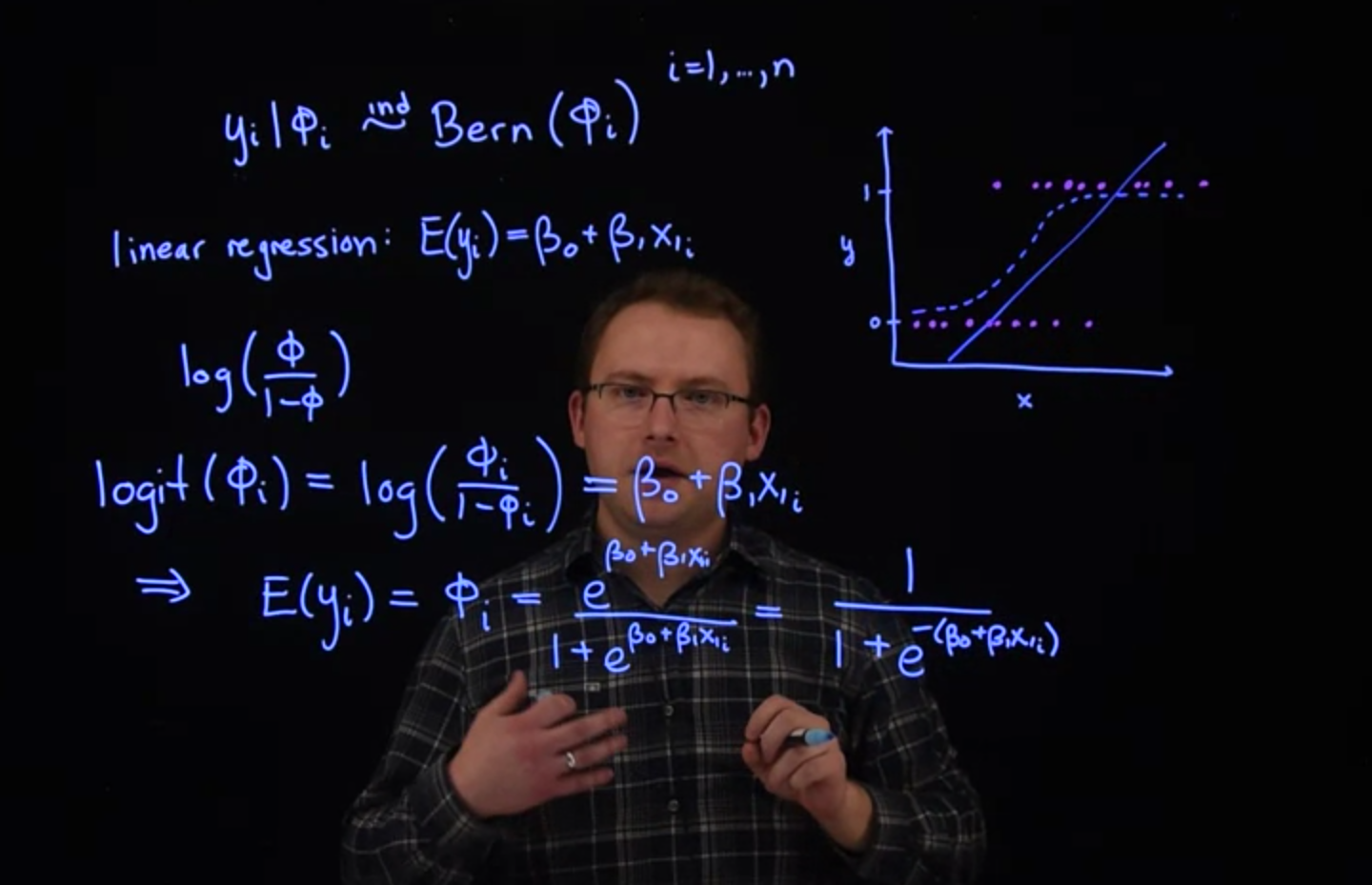
[Logistic regression is the preferred model when modelling a problem where the response variable is binary such as a classification or the outcome of a Bernoulli trial]{.mark}. In such the traditional least square fit suffers from a number of shortcomings. The main idea here is a log transform. However a naïve approach this transform imposes issues with 0 valued inputs since $log(0)=-\infty$
## Introduction to Logistic Regression :movie_camera: {#sec-intro-logistic-regression}
{#fig-intro-logistic-regression .column-margin width="53mm"}
### Data
\index{regression!logistic}
\index{dataset!urine}
For an example of logistic regression [**logistic regression**]{.column-margin}, we'll use the urine data set from the `boot` package in `R`. The response variable is `r`, which takes on values of 0 or 1. We will remove some rows from the data set which contain missing values.
```{r}
#| label: C2-L09-1
library("boot")
data("urine")
?urine
head(urine)
```
```{r}
#| label: C2-L09-2
dat = na.omit(urine) #<1>
```
1. drop missing values
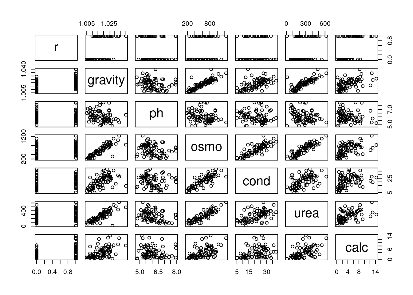
Let's look at pairwise scatter plots of the seven variables.
```{r}
#| label: C2-L09-3
pairs(dat)
```
One thing that stands out is that several of these variables are strongly correlated with one another. For example `gravity` and `osmo` appear to have a very close linear relationship. Collinearity between $x$ variables in linear regression models can cause trouble for statistical inference. [Two correlated variables will compete for the ability to predict the response variable, leading to unstable estimates. This is not a problem for prediction of the response, if prediction is the end goal of the model. But if our objective is to discover *how* the variables relate to the response, we should avoid collinearity.]{.mark}
::: {.callout-important}
## Collinearity and Multicollinearity {.unnumbered .unlisted}
\index{collinearity}
\index{multicollinearity}
When two covariates are highly correlated we call this relation **collinearity**.
When one covariate in a multiple regression model can be linearly predicted from the others with a substantial degree of accuracy we call this relation **multicollinearity**.
It is possible that no two pairs of a such a group of covariates are correlated.
In both cases this will lead to the *design matrix* being almost *singular.* Near singular matrices are a strong cause of instability in numerical calculations. Statistical this tends to lead to a model with inflated *standard errors* compared to models where we only keep the a subset where variables are neither **collinear** nor **multicollinear**. A consequence of this is that we will see a drop in *statistical significance* for these variables, which will make interpreting the model harder.
We have seen a few strategies ways to deal with these issues:
1. include `pair plot` in the exploratory data analysis phase.
2. picking subsets and checking DIC or,
3. variable selection using double exponential priors.
4. PCA creates independent covariates with a lower dimension with a trade of losing interpretability. See [@johnson2019applied p. 386] [@belsley1980 pp. 85-191] [@härdle2019]
5. Feature elimination based on combination of Variance inflation factors (VIF) [@sheather2009 p. 203]
:::
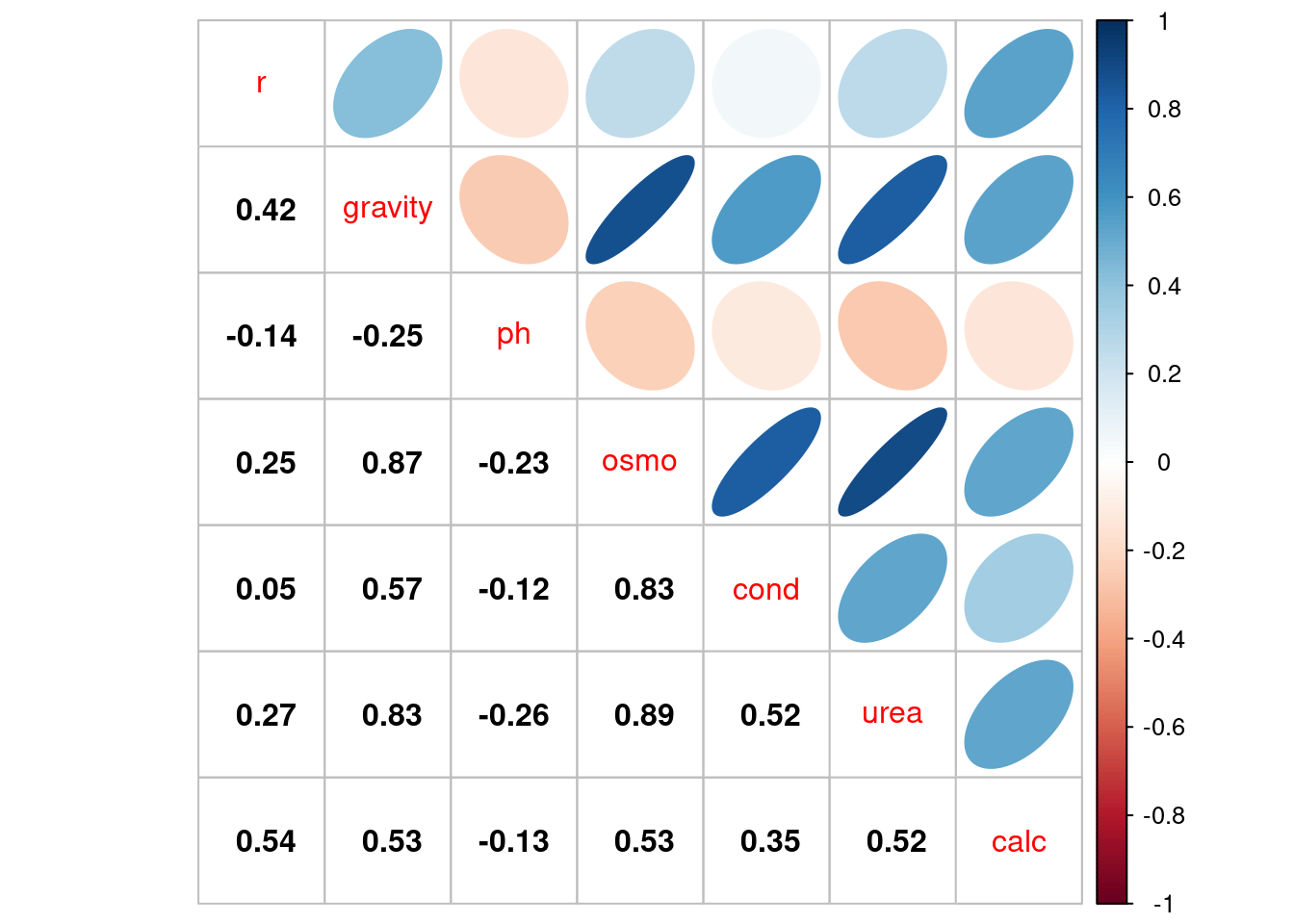
We can more formally estimate the correlation among these variables using the `corrplot` package.
```{r}
#| label: C2-L09-4
library("corrplot")
Cor = cor(dat)
corrplot(Cor, type="upper", method="ellipse", tl.pos="d")
corrplot(Cor, type="lower", method="number", col="black",
         add=TRUE, diag=FALSE, tl.pos="n", cl.pos="n")
```
### Variable selection
One primary goal of this analysis is to find out which variables are related to the presence of calcium oxalate crystals. This objective is often called "variable selection." We have already seen one way to do this: fit several models that include different sets of variables and see which one has the best DIC. Another way to do this is to use a linear model where the priors for the $\beta$ coefficients favor values near 0 (indicating a weak relationship). This way, the burden of establishing association lies with the data. If there is not a strong signal, we assume it doesn't exist.
Rather than tailoring a prior for each individual $\beta$ based on the scale its covariate takes values on, it is customary to subtract the mean and divide by the standard deviation for each variable.
```{r}
#| label: C2-L09-5
X = scale(dat[,-1], center=TRUE, scale=TRUE)
head(X[,"gravity"])
```
```{r}
#| label: C2-L09-6
colMeans(X)
```
```{r}
#| label: C2-L09-7
apply(X, 2, sd)
```
### Model
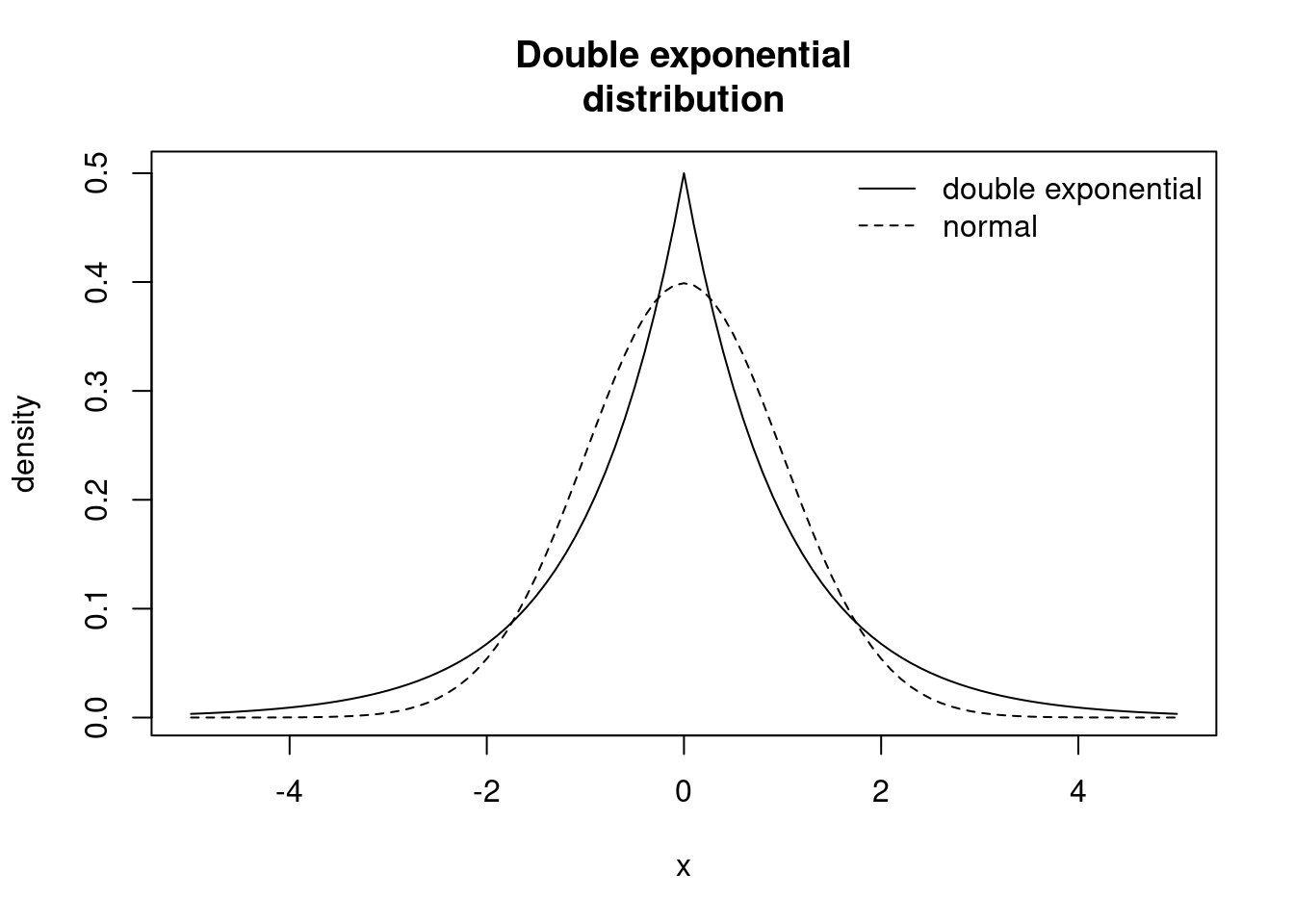
Our prior for the $\beta$ (which we'll call $b$ in the model) coefficients will be the double exponential (or Laplace) distribution, which as the name implies, is the exponential distribution with tails extending in the positive direction as well as the negative direction, with a sharp peak at 0. We can read more about it in the `JAGS` manual. The distribution looks like:
```{r}
#| label: C2-L09-8
ddexp = function(x, mu, tau) {
  0.5*tau*exp(-tau*abs(x-mu))
}
curve(ddexp(x, mu=0.0, tau=1.0), from=-5.0, to=5.0,
      ylab="density",
      main="Double exponential\ndistribution") # double exponential distribution
curve(dnorm(x, mean=0.0, sd=1.0), from=-5.0, to=5.0,
      lty=2, add=TRUE) # normal distribution
legend("topright",
      legend=c("double exponential", "normal"),
      lty=c(1,2), bty="n")
```
```{r}
#| label: C2-L09-9
library("rjags")
```
```{r}
#| label: C2-L09-10
mod1_string =
  " model {
    for (i in 1:length(y)) {
        y[i] ~ dbern(p[i])
        logit(p[i]) = int + b[1]*gravity[i] +
                            b[2]*ph[i] +
                            b[3]*osmo[i] +
                            b[4]*cond[i] +
                            b[5]*urea[i] +
                            b[6]*calc[i]
    }
    int ~ dnorm(0.0, 1.0/25.0)
    for (j in 1:6) {
        b[j] ~ ddexp(0.0, sqrt(2.0)) # has var 1.0
    }
} "

set.seed(92)
head(X)
data_jags = list(y=dat$r,
                 gravity=X[,"gravity"],
                 ph=X[,"ph"],
                 osmo=X[,"osmo"],
                 cond=X[,"cond"],
                 urea=X[,"urea"],
                 calc=X[,"calc"])
params = c("int", "b")

mod1 = jags.model(textConnection(mod1_string), data=data_jags, n.chains=3)
update(mod1, 1e3)
mod1_sim = coda.samples(model=mod1,
variable.names=params,
n.iter=5e3)
mod1_csim = as.mcmc(do.call(rbind, mod1_sim))
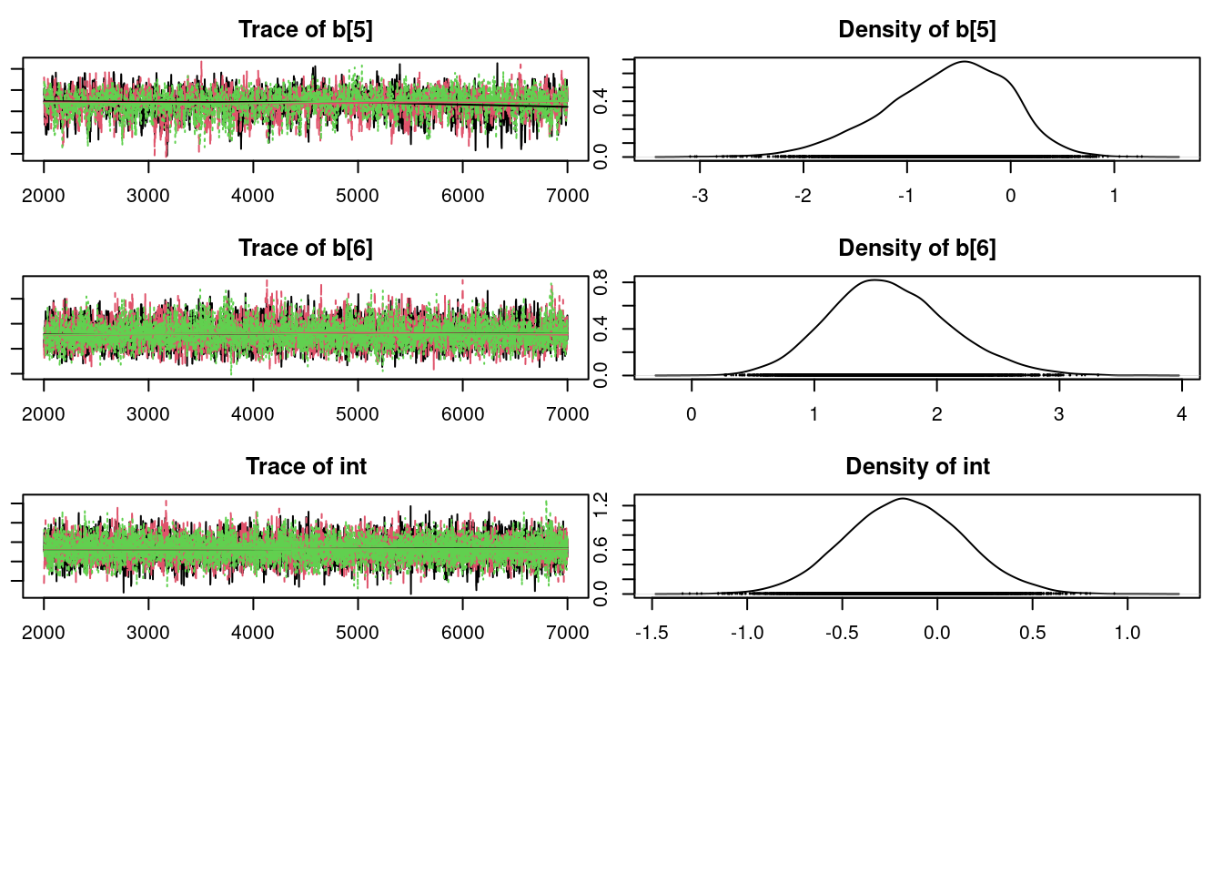
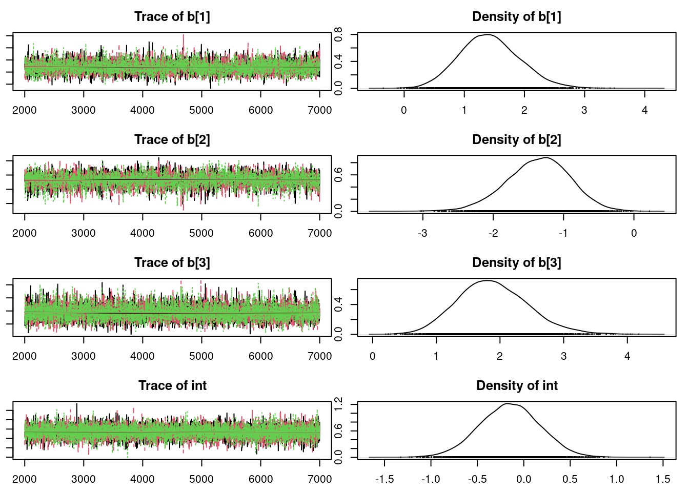
## convergence diagnostics
par(mar = c(2.5, 1, 2.5, 1))
plot(mod1_sim, ask=TRUE)
gelman.diag(mod1_sim)
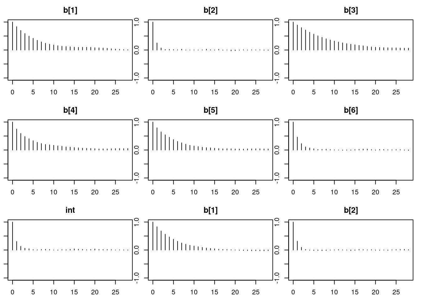
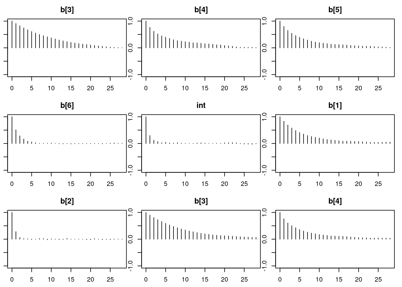
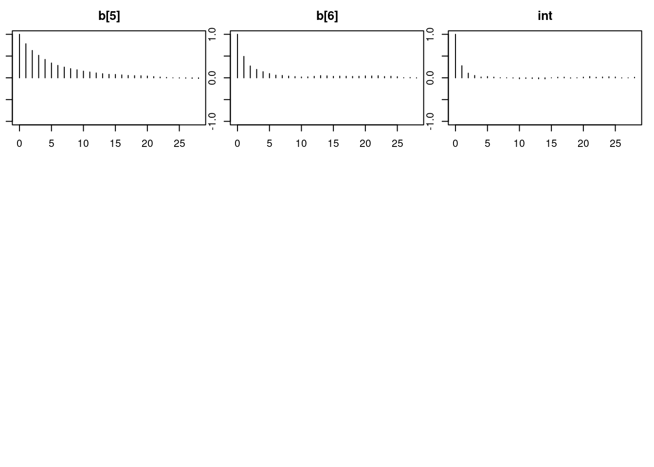
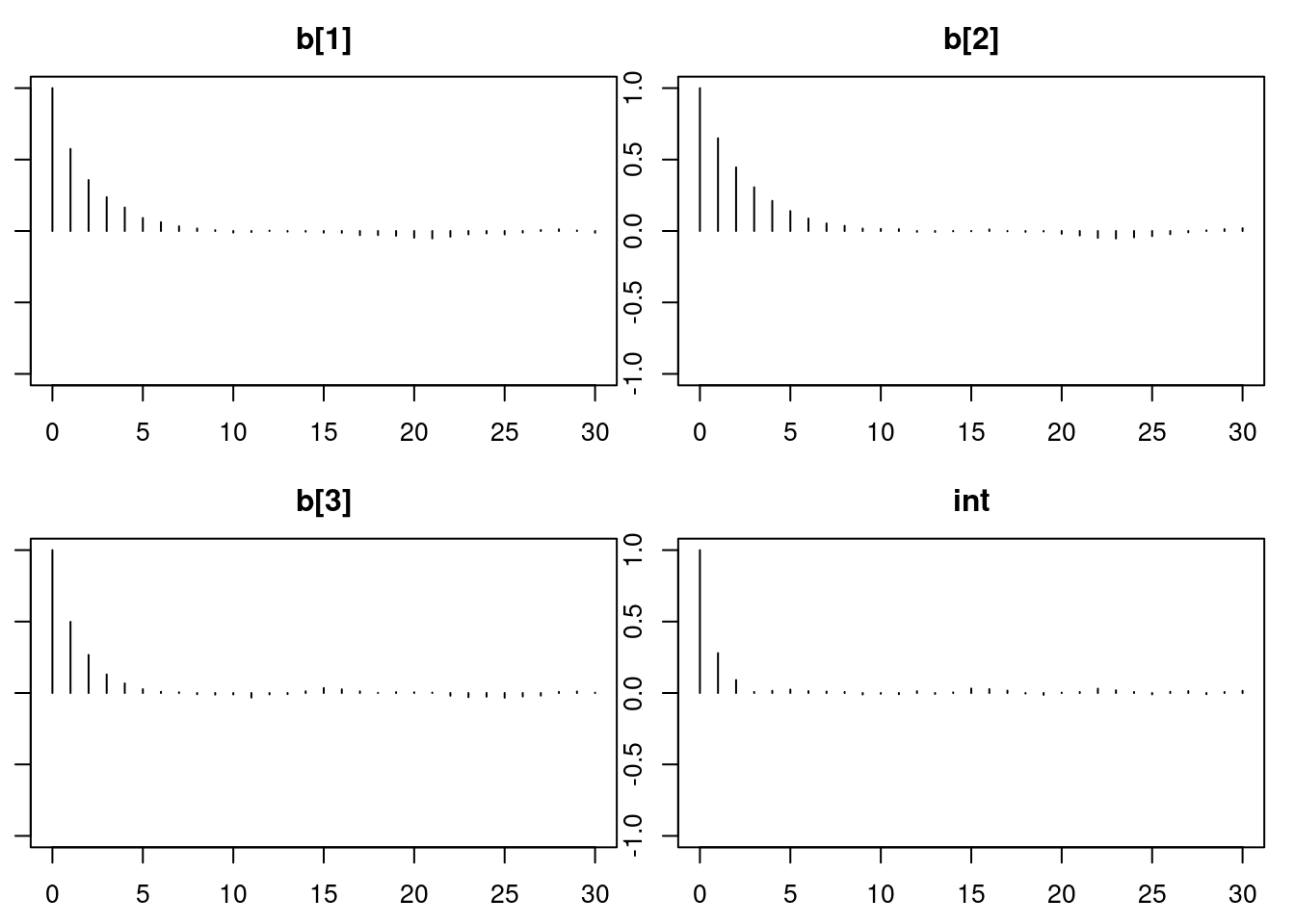
autocorr.diag(mod1_sim)
autocorr.plot(mod1_sim)
effectiveSize(mod1_sim)
## calculate DIC
dic1 = dic.samples(mod1, n.iter=1e3)
```
\index{model selection!DIC}
Let's look at the results.
```{r}
#| label: C2-L09-11
summary(mod1_sim)
```
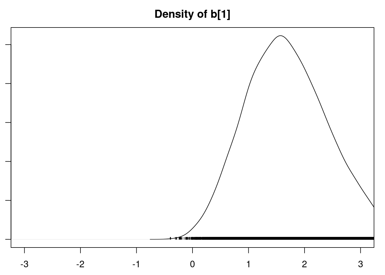
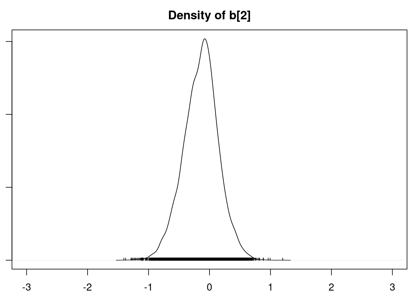
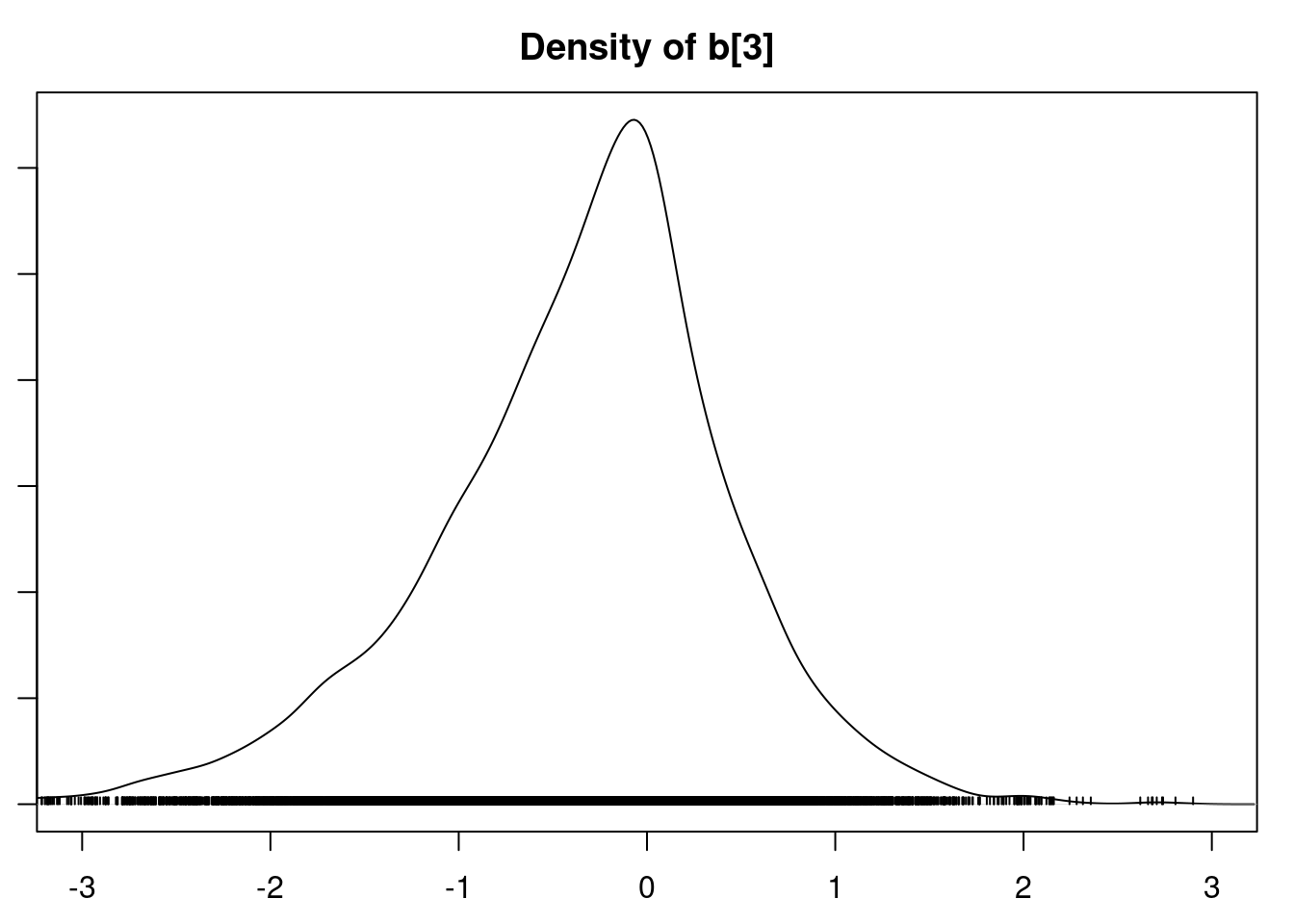
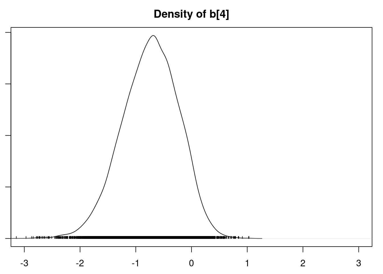
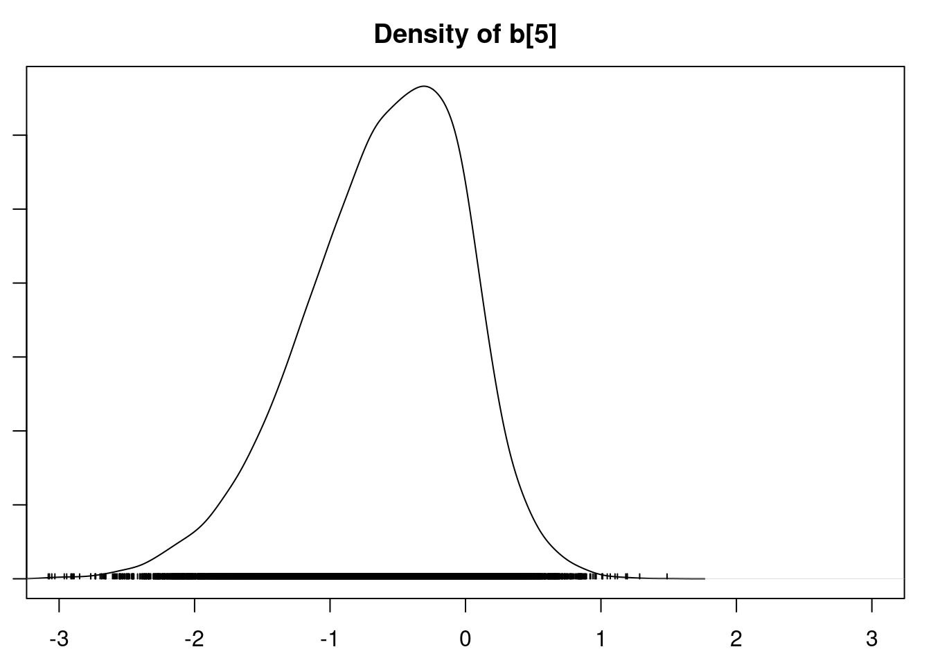
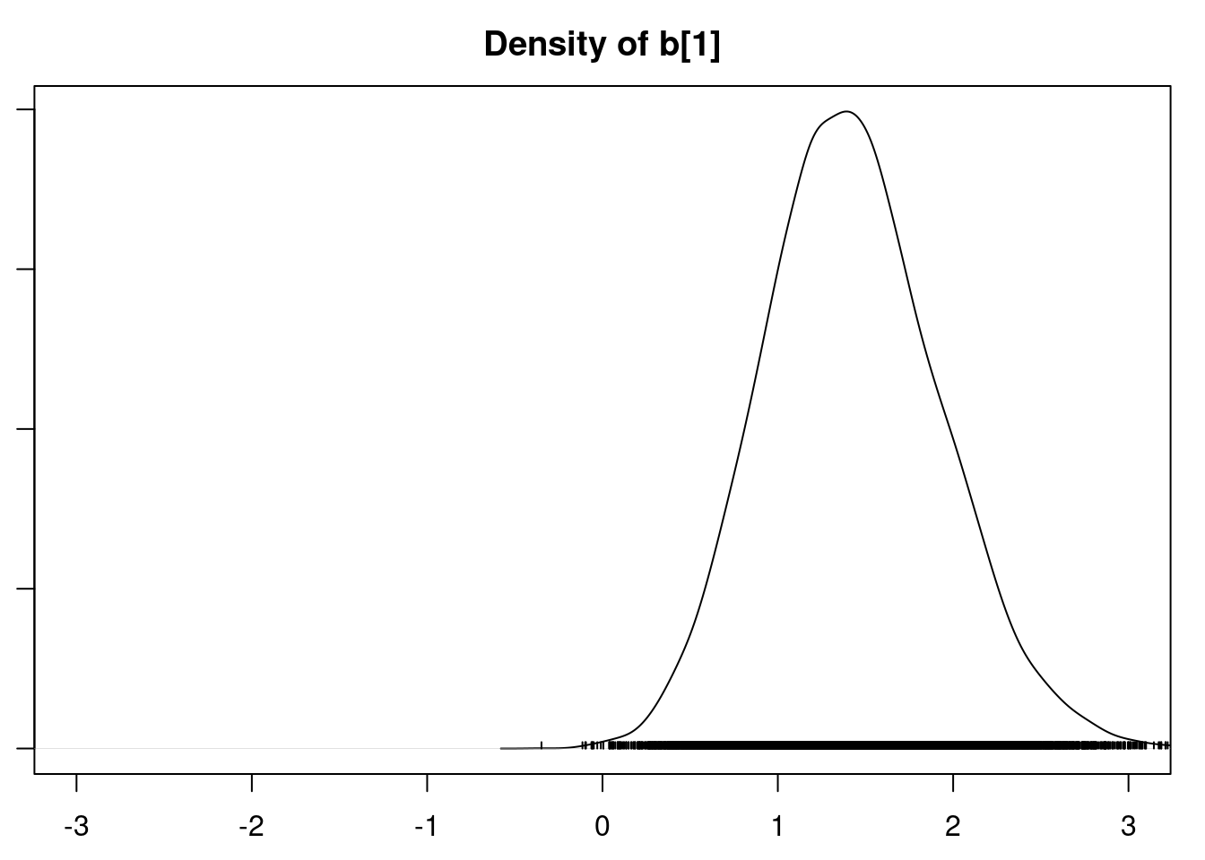
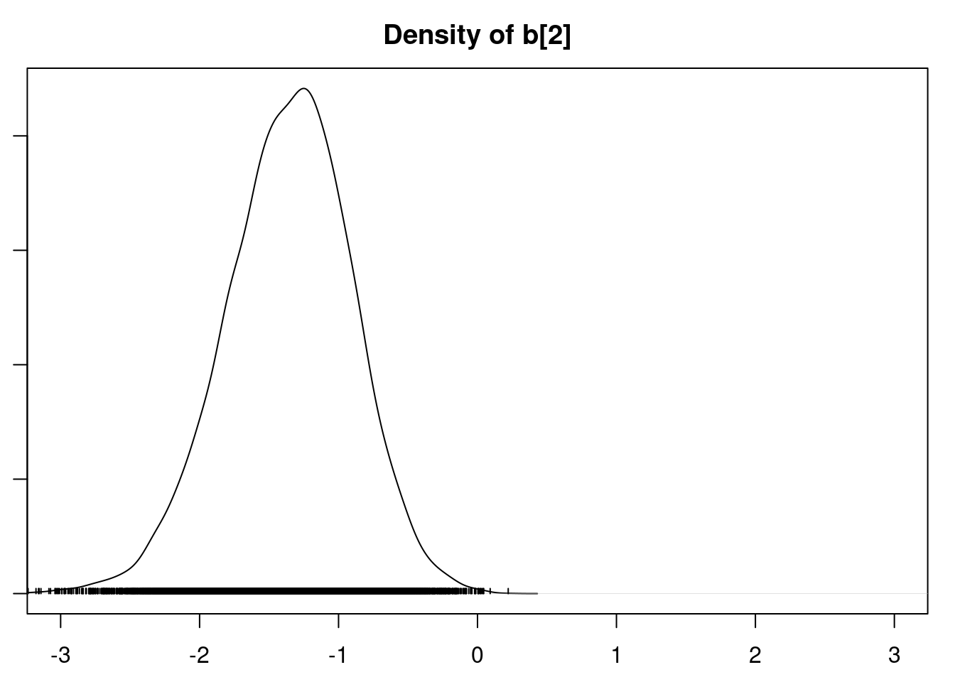
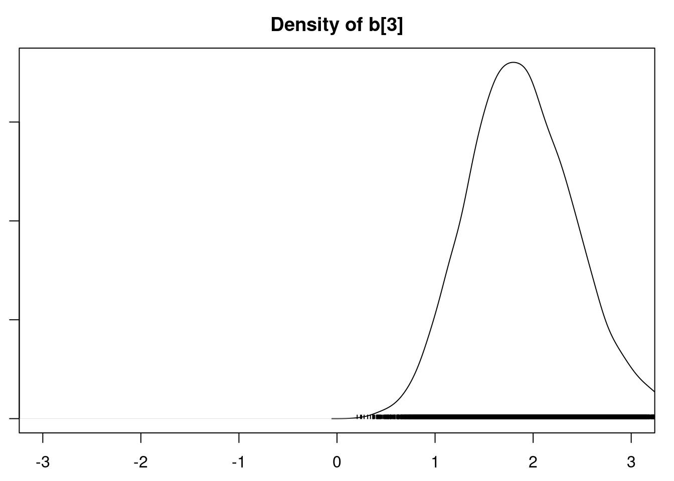
```{r}
#| label: C2-L09-12
#par(mfrow=c(3,2))
par(mar = c(2.5, 1, 2.5, 1))

densplot(mod1_csim[,1:6], xlim=c(-3.0, 3.0))
```
```{r}
#| label: C2-L09-13
colnames(X) # variable names
```
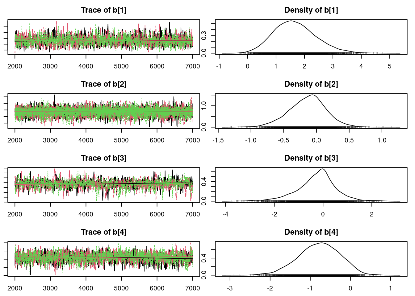
It is clear that the coefficients for variables `gravity`, `cond` (conductivity), and `calc` (calcium concentration) are not 0. The posterior distribution for the coefficient of `osmo` (osmolarity) looks like the prior, and is almost centered on 0 still, so we'll conclude that `osmo` is not a strong predictor of calcium oxalate crystals. The same goes for `ph`.
`urea` (urea concentration) appears to be a borderline case. However, if we refer back to our correlations among the variables, we see that `urea` is highly correlated with `gravity`, so we opt to remove it.
Our second model looks like this:
```{r}
#| label: C2-L09-14
mod2_string = " model {
    for (i in 1:length(y)) {
        y[i] ~ dbern(p[i])
        logit(p[i]) = int + b[1]*gravity[i] + b[2]*cond[i] + b[3]*calc[i]
    }
    int ~ dnorm(0.0, 1.0/25.0)
    for (j in 1:3) {
        b[j] ~ dnorm(0.0, 1.0/25.0) # noninformative for logistic regression
    }
} "

mod2 = jags.model(textConnection(mod2_string), data=data_jags, n.chains=3)
```
```{r}
#| label: C2-L09-15
update(mod2, 1e3)

mod2_sim = coda.samples(model=mod2,
                        variable.names=params,
                        n.iter=5e3)
mod2_csim = as.mcmc(do.call(rbind, mod2_sim))

par(mar = c(2.5, 1, 2.5, 1))
#plot(mod2_sim, ask=TRUE)
plot(mod2_sim)
gelman.diag(mod2_sim)
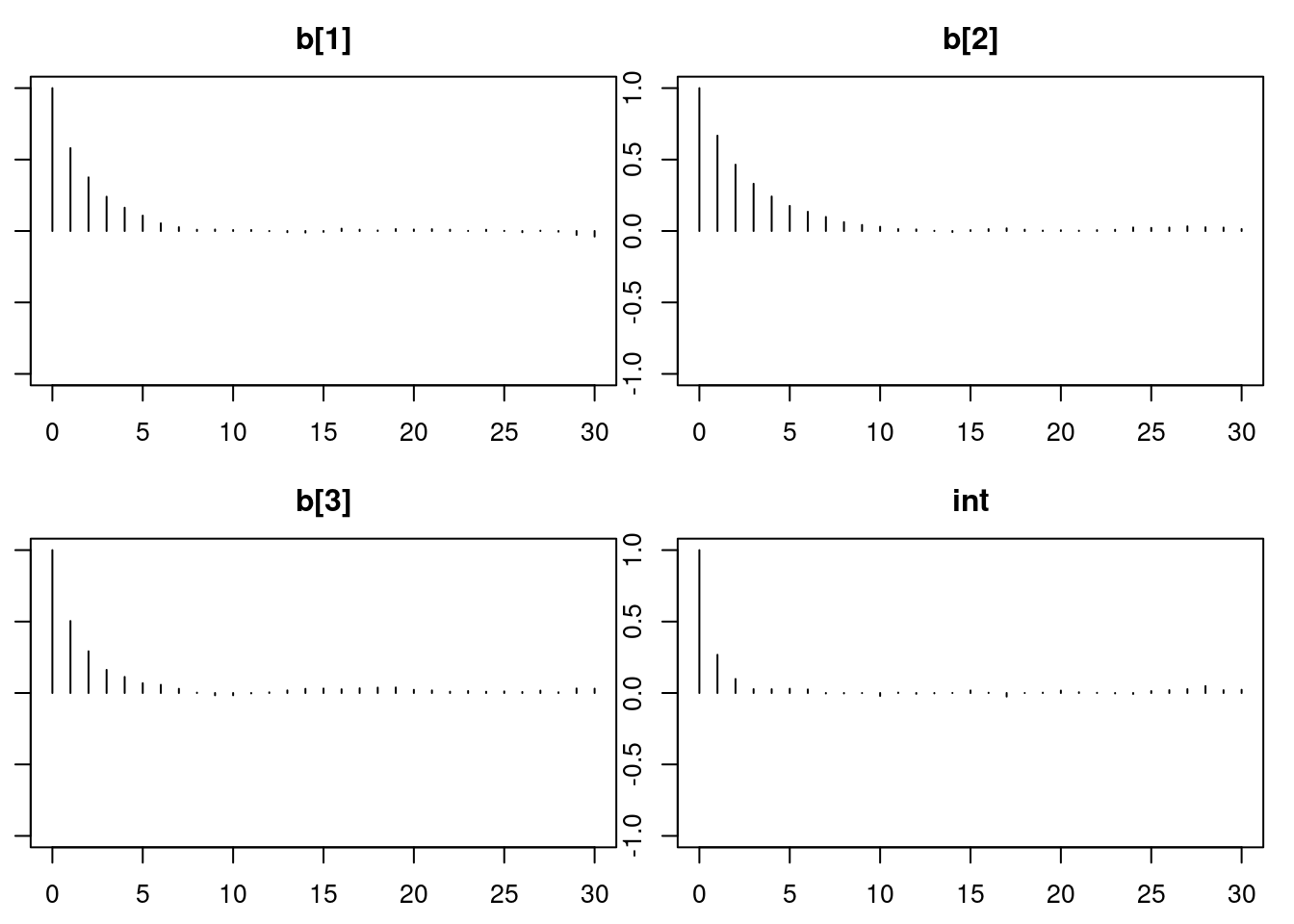
autocorr.diag(mod2_sim)
autocorr.plot(mod2_sim)
effectiveSize(mod2_sim)
dic2 = dic.samples(mod2, n.iter=1e3)
```
### Results
```{r}
#| label: C2-L09-16
dic1
```
```{r}
#| label: C2-L09-17
dic2
```
```{r}
#| label: C2-L09-18
summary(mod2_sim)
```
```{r}
#| label: C2-L09-19
HPDinterval(mod2_csim)
```
```{r}
#| label: C2-L09-20
#par(mfrow=c(3,1))
par(mar = c(2.5, 1, 2.5, 1))
densplot(mod2_csim[,1:3], xlim=c(-3.0, 3.0))
```
```{r}
#| label: C2-L09-21
colnames(X)[c(1,4,6)] # variable names
```
\index{Deviance information criterion}
\index{model selection!DIC}
The DIC is actually better for the first model. Note that we did change the prior between models, and generally we should not use the DIC to choose between priors. Hence comparing DIC between these two models may not be a fair comparison. Nevertheless, they both yield essentially the same conclusions. Higher values of `gravity` and `calc` (calcium concentration) are associated with higher probabilities of *calcium oxalate crystals*, while higher values of `cond` (conductivity) are associated with lower probabilities of *calcium oxalate crystals*.
There are more modeling options in this scenario, perhaps including transformations of variables, different priors, and interactions between the predictors, but we'll leave it to you to see if you can improve the model.