---
title: "Assessing Convergence - M2L5"
subtitle: "Bayesian Statistics: Techniques and Models"
description: "An overview of methods for assessing convergence in Markov Chain Monte Carlo simulations."
categories:
- Monte Carlo Estimation
keywords:
- convergence diagnostics
- trace plots
- autocorrelation
- effective sample size
- Gelman-Rubin diagnostic
- R programming
- statistical modeling
- Bayesian statistics
---
## Convergence diagnostics {#sec-convergence-diagnostics}
In the previous two lessons, we have demonstrated ways you can simulate a Markov chain whose stationary distribution is the target distribution (usually the posterior). Before using the simulated chain to obtain Monte Carlo estimates, we should first ask ourselves: Has our simulated Markov chain converged to its stationary distribution yet? Unfortunately, this is a difficult question to answer, but we can do several things to investigate.
### Trace plots {#sec-trace-plots}
Our first visual tool for assessing chains is the trace plot. A trace plot shows the history of a parameter value across iterations of the chain. It shows you precisely where the chain has been exploring.
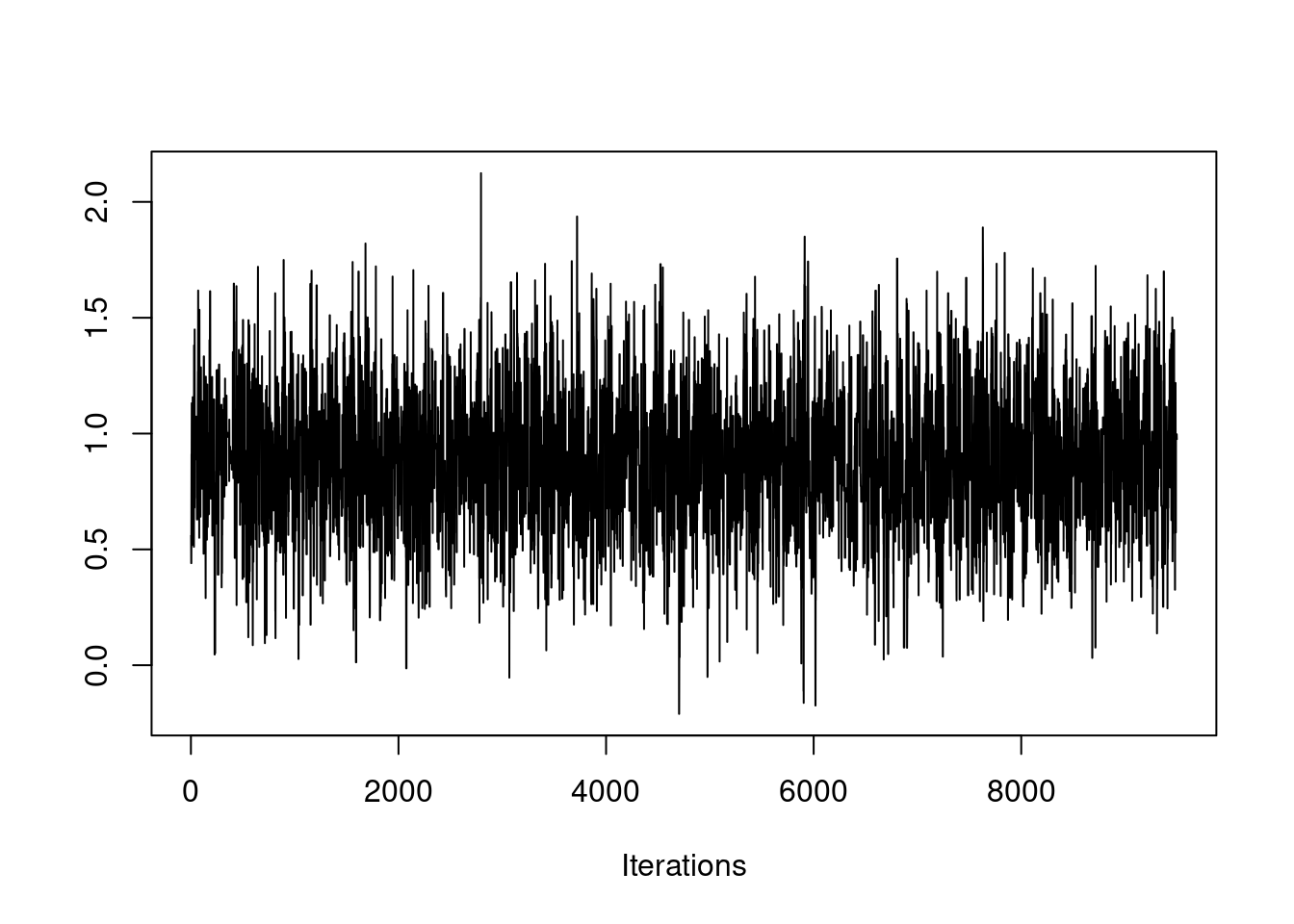
First, let's talk about what a chain should look like. Here is an example of a chain that has most likely converged.
```{r}
#| label: C2-L06-1
source('mh.r')
library("coda")
set.seed(61)
post0 = mh(n=n, ybar=ybar, n_iter=10e3, mu_init=0.0, cand_sd=0.9)
coda::traceplot(as.mcmc(post0$mu[-c(1:500)]))
```
If the chain is stationary, it should not be showing any long-term trends. The average value for the chain should be roughly flat. It should not be wandering as in this example:
```{r}
#| label: C2-L06-2
set.seed(61)
post1 = mh(n=n, ybar=ybar, n_iter=1e3, mu_init=0.0, cand_sd=0.04)
coda::traceplot(as.mcmc(post1$mu[-c(1:500)]))
```
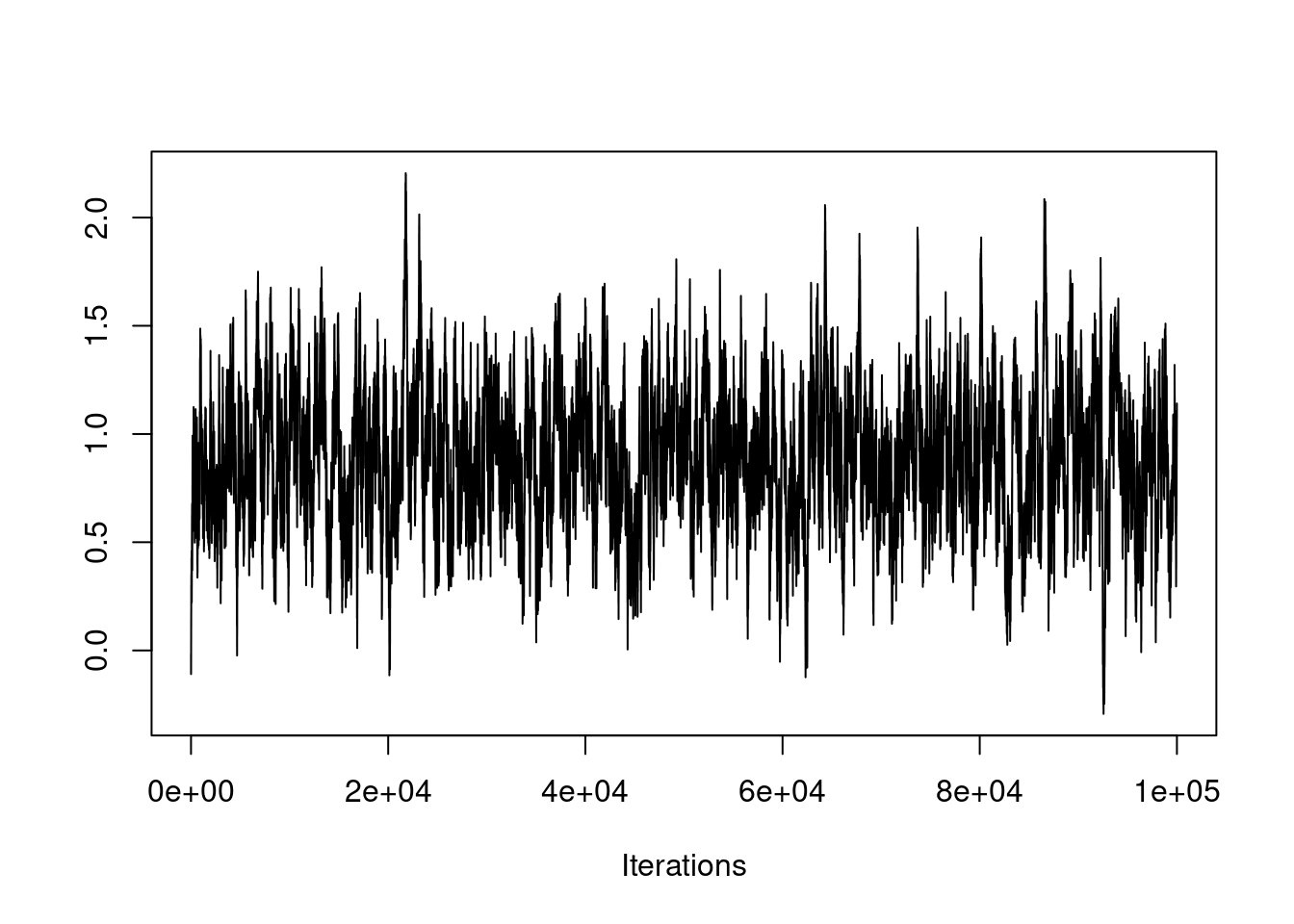
If this is the case, you need to run the chain many more iterations, as seen here:
```{r}
#| label: C2-L06-3
set.seed(61)
post2 = mh(n=n, ybar=ybar, n_iter=100e3, mu_init=0.0, cand_sd=0.04)
coda::traceplot(as.mcmc(post2$mu))
```
The chain appears to have converged at this much larger time scale.
### Monte Carlo effective sample size
\index{MCMC!effective sample size}
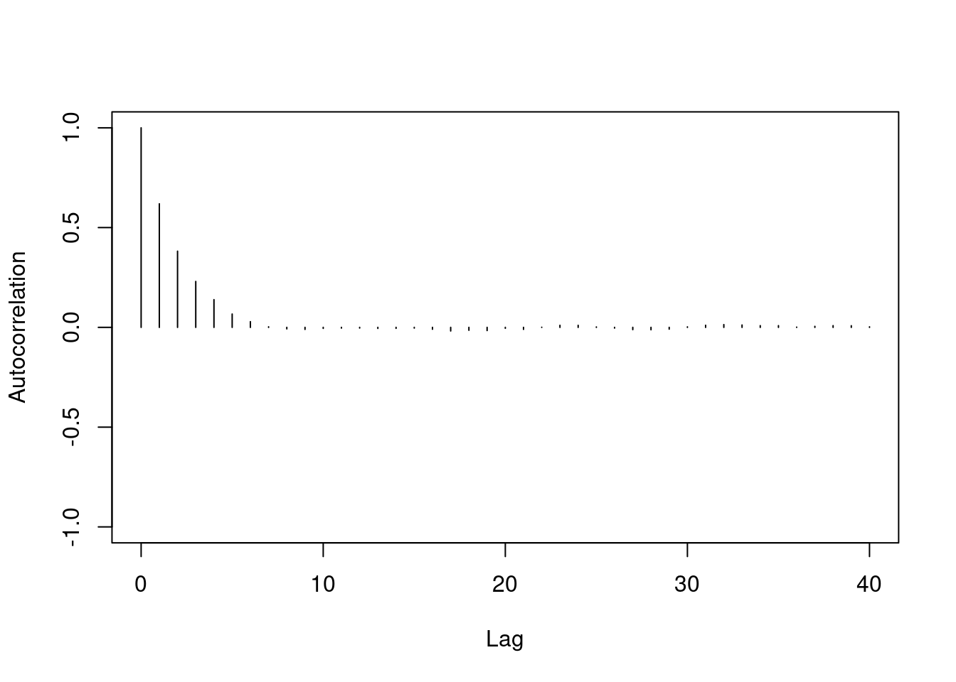
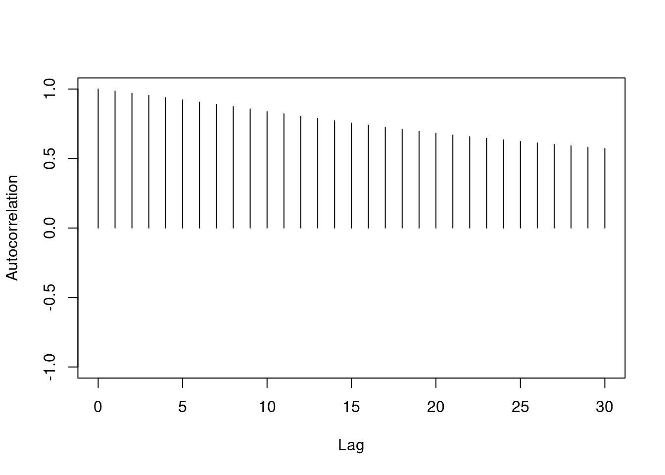
One major difference between the two chains we've looked at is the level of autocorrelation in each. Autocorrelation is a number between $-1$ and $+1$ which measures how linearly dependent the current value of the chain is on past values (called lags). We can see this with an autocorrelation plot:
```{r}
#| label: C2-L06-4
coda::autocorr.plot(as.mcmc(post0$mu))
```
```{r}
#| label: C2-L06-5
coda::autocorr.plot(as.mcmc(post1$mu))
```
```{r}
#| label: C2-L06-6
coda::autocorr.diag(as.mcmc(post1$mu))
```
Autocorrelation is important because it tells us how much information is available in our Markov chain. Sampling 1000 iterations from a highly correlated Markov chain yields less information about the stationary distribution than we would obtain from 1000 samples *independently* drawn from the stationary distribution.
Autocorrelation is a major component in calculating the Monte Carlo effective sample size of your chain. The Monte Carlo effective sample size is how many *independent* samples from the stationary distribution you would have to draw to have equivalent information in your Markov chain. Essentially it is the $m$ (sample size) we chose in the lesson on Monte Carlo estimation.
```{r}
#| label: C2-L06-7
str(post2) # contains 100,000 iterations
```
```{r}
#| label: C2-L06-8
coda::effectiveSize(as.mcmc(post2$mu)) # effective sample size of ~350
```
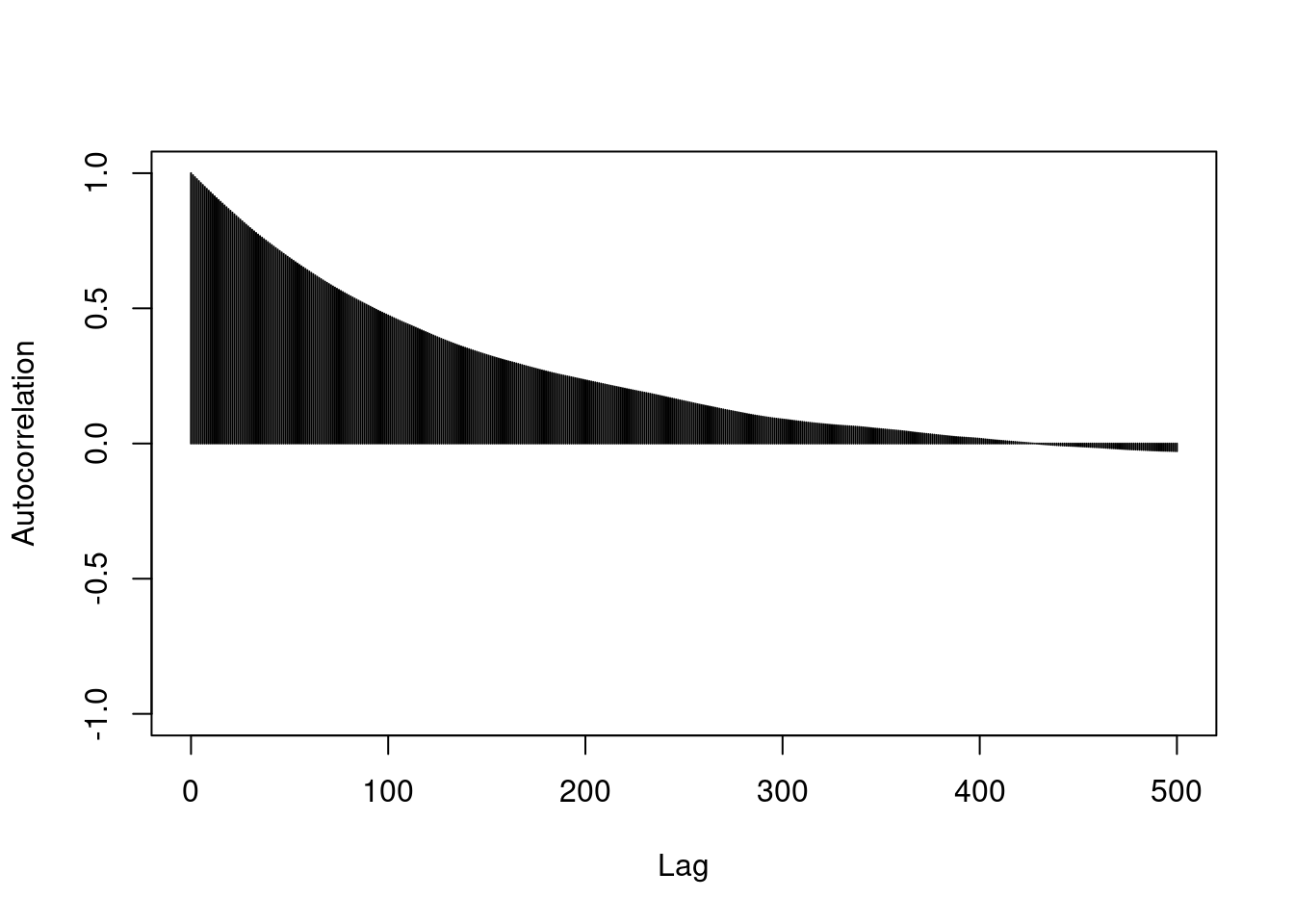
```{r}
#| label: C2-L06-9
## thin out the samples until autocorrelation is essentially 0. This will leave you with approximately independent samples. The number of samples remaining is similar to the effective sample size.
coda::autocorr.plot(as.mcmc(post2$mu), lag.max=500)
```
```{r}
#| label: C2-L06-10
thin_interval = 400 # how far apart the iterations are for autocorrelation to be essentially 0.
thin_indx = seq(from=thin_interval, to=length(post2$mu), by=thin_interval)
head(thin_indx)
```
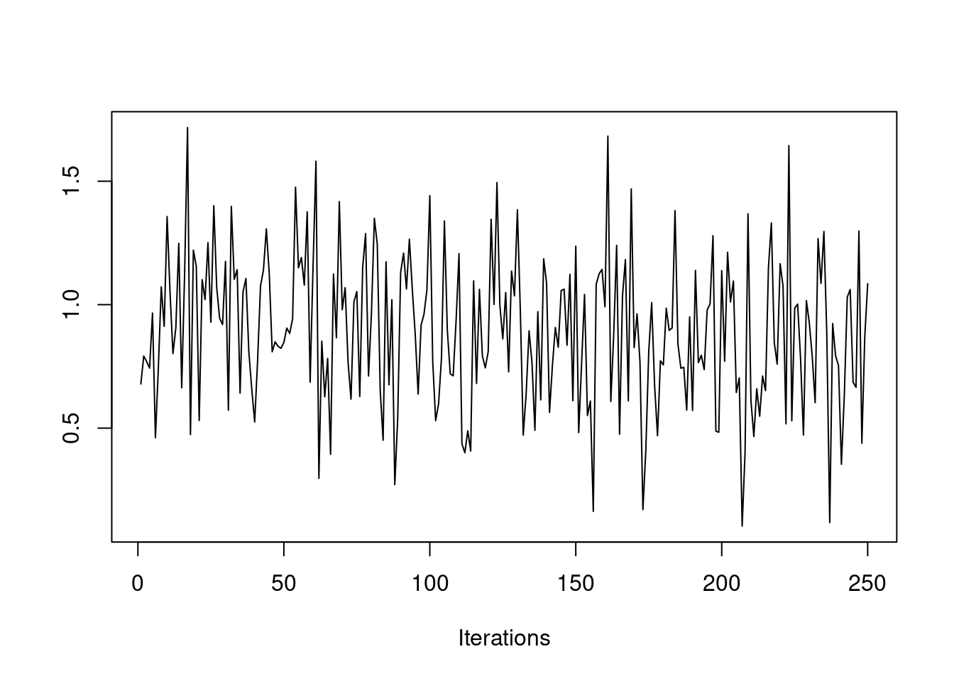
```{r}
#| label: C2-L06-11
post2mu_thin = post2$mu[thin_indx]
traceplot(as.mcmc(post2$mu))
```
```{r}
#| label: C2-L06-12
traceplot(as.mcmc(post2mu_thin))
```
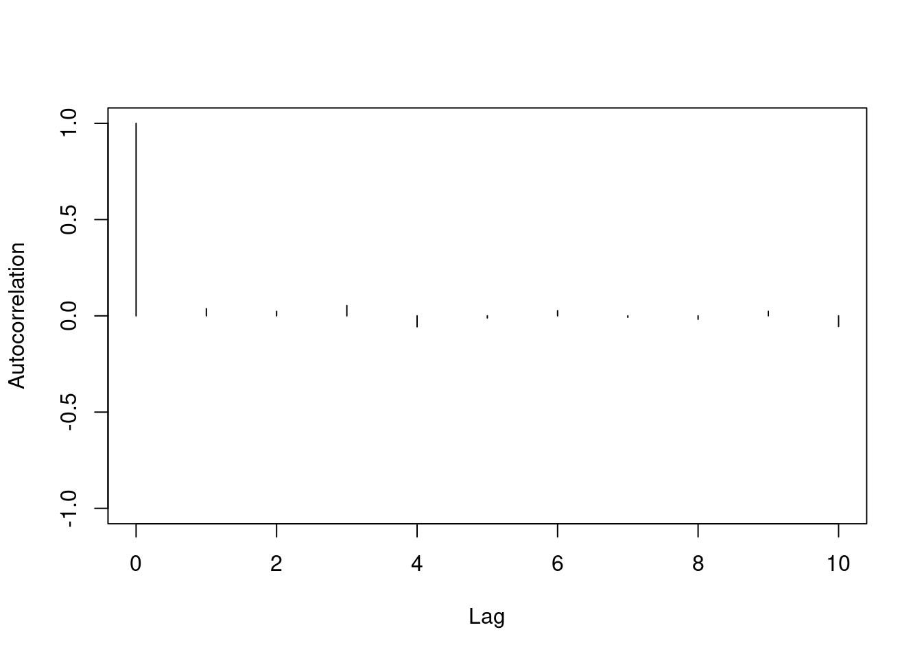
```{r}
#| label: C2-L06-13
coda::autocorr.plot(as.mcmc(post2mu_thin), lag.max=10)
```
```{r}
#| label: C2-L06-14
effectiveSize(as.mcmc(post2mu_thin))
```
```{r}
#| label: C2-L06-15
length(post2mu_thin)
```
```{r}
#| label: C2-L06-16
str(post0) # contains 10,000 iterations
```
```{r}
#| label: C2-L06-17
coda::effectiveSize(as.mcmc(post0$mu)) # effective sample size of ~2,500
```
```r
?effectiveSize
```
The chain from `post0` has 10,000 iterations, but an effective sample size of about 2,500. That is, this chain essentially provides the equivalent of 2,500 independent Monte Carlo samples.
Notice that the chain from `post0` has 10 times fewer iterations than for `post2`, but its Monte Carlo effective sample size is about seven times greater than the longer (more correlated) chain. We would have to run the correlated chain for 700,000+ iterations to get the same amount of information from both chains.
\index{MCMC!Raftery and Lewis diagnostic}
\index{MCMC!effective sample size}
It is usually a good idea to check the Monte Carlo effective sample size of your chain. If all you seek is a posterior mean estimate, then an effective sample size of a few hundred to a few thousand should be enough. However, if you want to create something like a 95% posterior interval, you may need many thousands of effective samples to produce a reliable estimate of the outer edges of the distribution. The number you need can be quickly calculated using the Raftery and Lewis diagnostic.
```r
raftery.diag(as.mcmc(post0$mu))
```
```{r}
#| label: C2-L06-18
raftery.diag(as.mcmc(post0$mu), q=0.005, r=0.001, s=0.95)
```
```{r}
#| label: C2-L06-19
##
## Quantile (q) = 0.005
## Accuracy (r) = +/- 0.001
## Probability (s) = 0.95
##
## You need a sample size of at least 19112 with these values of q, r and s
```
```{r}
#| label: C2-L06-20
?raftery.diag
```
In the case of the first chain from `post0`, it looks like we would need about 3,700 effective samples to calculate reliable 95% intervals. With the autocorrelation in the chain, that requires about 13,200 total samples. If we wanted to create reliable 99% intervals, we would need at least 19,100 total samples.
## Burn-in
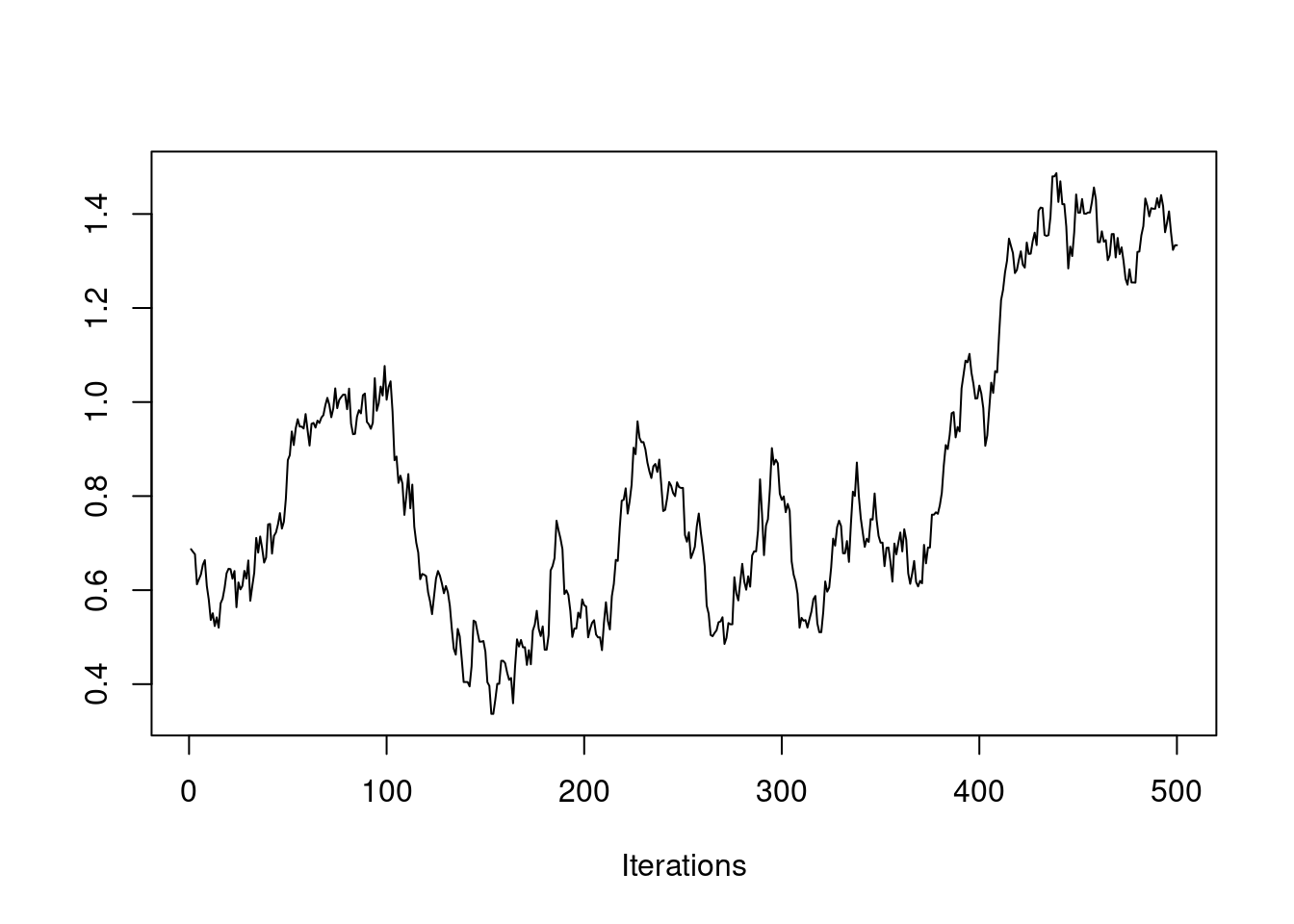
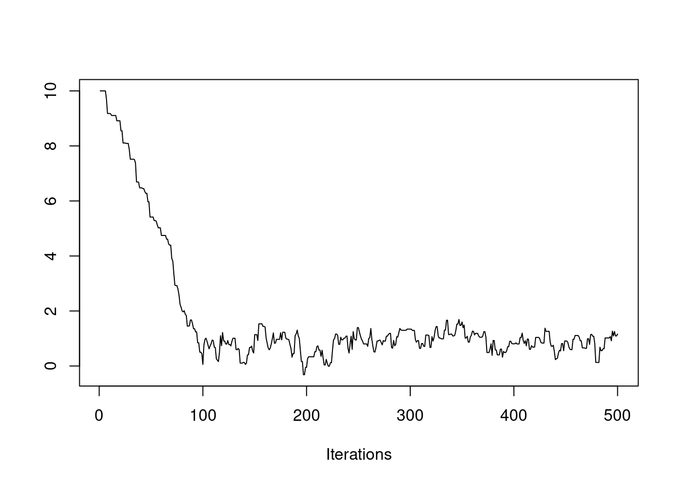
We have also seen how the initial value of the chain can affect how quickly the chain converges. If our initial value is far from the bulk of the posterior distribution, then it may take a while for the chain to travel there. We saw this in an earlier example.
```{r}
#| label: C2-L06-21
set.seed(62)
post3 = mh(n=n, ybar=ybar, n_iter=500, mu_init=10.0, cand_sd=0.3)
coda::traceplot(as.mcmc(post3$mu))
```
Clearly, the first 100 or so iterations do not reflect draws from the stationary distribution, so they should be discarded before we use this chain for Monte Carlo estimates. This is called the "burn-in" period. You should always discard early iterations that do not appear to be coming from the stationary distribution. Even if the chain appears to have converged early on, it is safer practice to discard an initial burn-in.
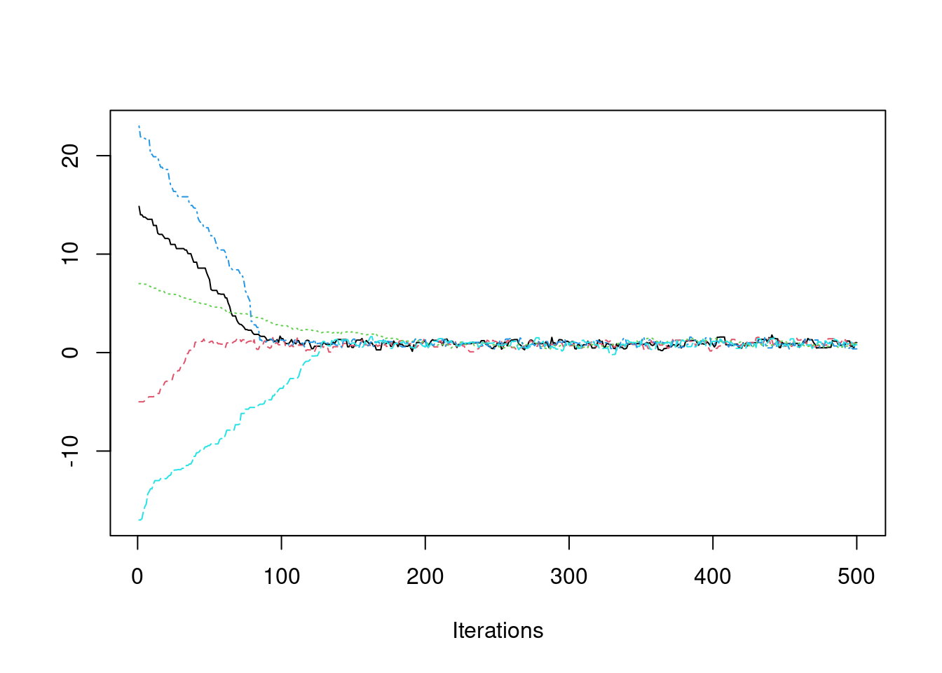
### Multiple chains, Gelman-Rubin
If we want to be more confident that we have converged to the true stationary distribution, we can simulate multiple chains, each with a different starting value.
```{r}
#| label: C2-L06-22
set.seed(61)

nsim = 500
post1 = mh(n=n, ybar=ybar, n_iter=nsim, mu_init=15.0, cand_sd=0.4)
post1$accpt
```
```{r}
#| label: C2-L06-23
post2 = mh(n=n, ybar=ybar, n_iter=nsim, mu_init=-5.0, cand_sd=0.4)
post2$accpt
```
```{r}
#| label: C2-L06-24
post3 = mh(n=n, ybar=ybar, n_iter=nsim, mu_init=7.0, cand_sd=0.1)
post3$accpt
```
```{r}
#| label: C2-L06-25
post4 = mh(n=n, ybar=ybar, n_iter=nsim, mu_init=23.0, cand_sd=0.5)
post4$accpt
```
```{r}
#| label: C2-L06-26
post5 = mh(n=n, ybar=ybar, n_iter=nsim, mu_init=-17.0, cand_sd=0.4)
post5$accpt
```
```{R}
#| label: C2-L06-27
pmc = mcmc.list(as.mcmc(post1$mu), as.mcmc(post2$mu),
                as.mcmc(post3$mu), as.mcmc(post4$mu), as.mcmc(post5$mu))
str(pmc)
```
```{r}
#| label: C2-L06-28
coda::traceplot(pmc)
```
It appears that after about iteration 200, all chains are exploring the stationary (posterior) distribution.
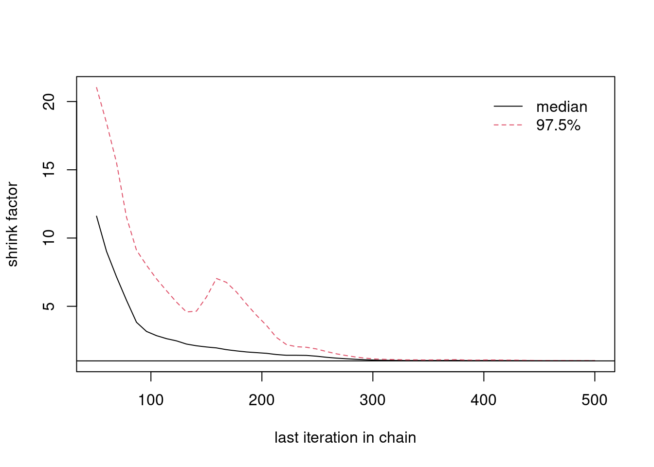
We can back up our visual results with the Gelman Rubin diagnostic. \index{Gelman Rubin diagnostic}
This diagnostic statistic calculates the variability within chains, comparing that to the variability between chains.
If all chains have converged to the stationary distribution, the variability between chains should be relatively small, and the potential scale reduction factor, reported by the the diagnostic, should be close to one.
If the values are much higher than one, then we would conclude that the chains have not yet converged.
```{r}
#| label: C2-L06-29
coda::gelman.diag(pmc)
```
```{r}
#| label: C2-L06-30
coda::gelman.plot(pmc)
```
```{r}
#| label: C2-L06-31
?gelman.diag
```
\index{shrink factor}
\index{scale reduction factor}
From the plot, we can see that if we only used the first 50 iterations, the potential scale reduction factor or "shrink factor" would be close to 10, indicating that the chains have not converged. But after about iteration 300, the "shrink factor" is essentially one, indicating that by then, we have probably reached convergence. Of course, we shouldn't stop sampling as soon as we reach convergence. Instead, this is where we should begin saving our samples for Monte Carlo estimation.
### Monte Carlo estimation
If we are reasonably confident that our Markov chain has converged, then we can go ahead and treat it as a Monte Carlo sample from the posterior distribution. Thus, we can use the techniques from Lesson 3 to calculate posterior quantities like the posterior mean and posterior intervals from the samples directly.
```{r}
#| label: C2-L06-32
nburn = 1000 # remember to discard early iterations
post0$mu_keep = post0$mu[-c(1:1000)]
summary(as.mcmc(post0$mu_keep))
```
```{r}
#| label: C2-L06-33
mean(post0$mu_keep > 1.0) # posterior probability that mu > 1.0
```