69 The EM algorithm for Mixture Models

69.1 Infer parameter of mixture of exponential and long normal for lifetime of fuses

NoteInstructions

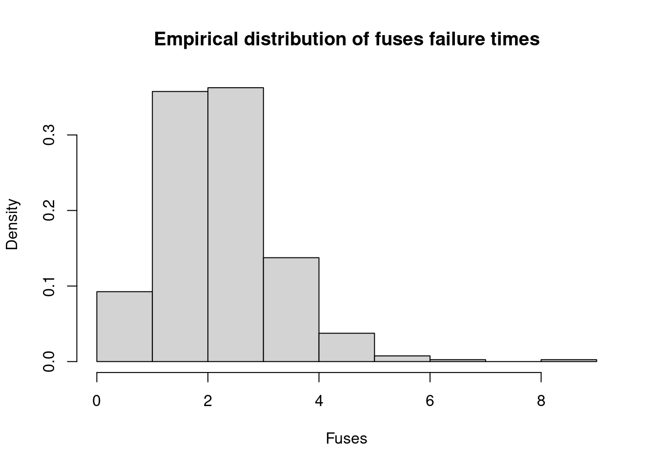
Data on the lifetime (in years) of fuses produced by the ACME Corporation is available in the file fuses.csv:

In order to characterize the distribution of the lifetimes, it seems reasonable to fit to the data a two-component mixture of the form:

f(x)=wλexp{−λx}+(1−w) \frac{1}{\sqrt{2\pi}\tau x} \exp{− \frac{(log(x)−μ)^{2}}{2τ^{2}}}, \quad x > 0. \tag{69.1}

where w is the weight associated with the exponential distribution, \lambda is the rate of the exponential distribution, and \text{LN}(\mu, \tau) is a log-normal distribution with mean \mu and standard deviation \tau.

• Modify code to Generate n observations from a mixture of two Gaussian # distributions into code to sample 100 random numbers from a mixture of 4 exponential distributions with means 1, 4, 7 and 10 and weights 0.3, 0.25, 0.25 and 0.2, respectively.
• Use these sample to approximate the mean and variance of the mixture.

## Clear the environment and load required libraries
rm(list=ls())
set.seed(81196)    # So that results are reproducible (same simulated data every time)

# Load the data
fuses <- read.csv("data/fuses.csv",header=FALSE)
x <- fuses$V1
n <- length(x) # Number of observations

# how many rows in the data
nrow(fuses)

[1] 400

# how many zeros in x
sum(x==0)

[1] 0

# almost half of the data is zeros!

par(mfrow=c(1,1))
xx.true = seq(0, max(x), by=1)
hist(x, freq=FALSE, xlab="Fuses", ylab="Density", main="Empirical distribution of fuses failure times")

KK = 2                             # Number of components
w     = 0.05                        # Assign equal weight to each component to start with
#mu = rnorm(1,mean(log(x)), sd(log(x)))
mu = mean(log(x))
tau = sd(log(x))
lambda = 20 / mean(x)

s  = 0              # s_tep counter
sw = FALSE          # sw_itch to stop the algorithm
QQ = -Inf           # the Q function (log-likelihood function)
QQ.out = NULL       # the Q function values
epsilon = 10^(-5)   # the stopping criterion for the algorithm

trace <- data.frame(iter=0, w=w, lambda=lambda, mu=mu, tau=tau)

while(!sw){ ##Checking convergence

  ## E step
  v = array(0, dim=c(n,KK))
  for(i in 1:n){
    v[i,1] = log(w)   + dexp(x[i], rate=lambda, log=TRUE)
    v[i,2] = log(1-w) + dlnorm(x[i], mu, tau, log=TRUE)    
    v[i,]  = exp(v[i,] - max(v[i,]))/sum(exp(v[i,] - max(v[i,]))) 
  }

  ## M step  
  w      = mean(v[,1])  # Weights
  lambda = sum(v[,1]) / sum(v[,1] * x)  # Lambda (rate)
  mu     = sum(v[,2] * log(x)) / sum(v[,2]) # Mean
  tau    = sqrt(sum(v[,2] * (log(x) - mu)^2) / sum(v[,2])) # Tau (standard deviation)
  
  # collect trace of parameters 
  trace  =  rbind(trace, data.frame(iter=s, w=w, lambda=lambda, mu=mu, tau=tau))

  ## Check convergence
  QQn = 0
  #vectorized version
  log_lik_mat = v[,1]*(log(w)   + dexp(x, lambda, log=TRUE)) +
                v[,2]*(log(1-w) + dlnorm(x, mu, tau, log=TRUE))
  QQn = sum(log_lik_mat)
  if(abs(QQn-QQ)/abs(QQn)<epsilon){
    sw=TRUE
  }
  QQ = QQn
  QQ.out = c(QQ.out, QQ)
  s = s + 1
  print(paste(s, QQn))
}

[1] "1 -621.636631915928"
[1] "2 -576.564676680329"
[1] "3 -562.326030957339"
[1] "4 -558.240693010161"
[1] "5 -559.062812699431"
[1] "6 -560.433982999852"
[1] "7 -561.504096778213"
[1] "8 -562.257984979008"
[1] "9 -562.779349634224"
[1] "10 -563.139561270939"
[1] "11 -563.389080841182"
[1] "12 -563.562415697134"
[1] "13 -563.683109594057"
[1] "14 -563.767298770739"
[1] "15 -563.826100698272"
[1] "16 -563.867209281663"
[1] "17 -563.895967519019"
[1] "18 -563.916095326952"
[1] "19 -563.930187401928"
[1] "20 -563.94005598844"
[1] "21 -563.946968029888"
[1] "22 -563.951809840896"

next report the MLE parameters of the model.

# Report the MLE parameters
cat("w =", round(w, 2), "lambda =", round(lambda, 2), "mu =", round(mu, 2),"tau =", round(tau, 2))

w = 0.09 lambda = 3.05 mu = 0.78 tau = 0.38