---
date: 2025-07-07
subtitle: "Bayesian Statistics - Capstone Project"
description: "Capstone Project: Bayesian Conjugate Analysis for Autogressive Time Series Models"
categories:
- Bayesian Statistics
- Capstone Project
keywords:
- Time Series
execute:
freeze: true # never re-render during project render
---
## Location and scale mixture of AR model {#sec-capstone-lsm}
In this part, we will extend the **location mixture** of AR models to the **location and scale mixture** of AR models. We will show the derivation of the Gibbs sampler for the model parameters as well as the R code for the full posterior inference.
### The Model
The location and scale mixture of AR($p$) model for the data can be written hierarchically as follows:
$$
\begin{aligned}
&y_t\sim\sum_{k=1}^K\omega_kN(\mathbf{f}^T_t\boldsymbol{\beta}_k,\nu_k),\quad \mathbf{f}^T_t=(y_{t-1},\cdots,y_{t-p})^T,\quad t=p+1,\cdots,T\\
&\omega_k\sim Dir(a_1,\cdots,a_k),\quad \boldsymbol{\beta}_k\sim N(\mathbf{m}_0,\nu_k\mathbf{C}_0),\quad \nu_k\sim IG(\frac{n_0}{2},\frac{d_0}{2})
\end{aligned}
$$ {#eq-capstone-ls-arp-mixture}
Introducing latent configuration variable $L_t \in \{1,2,\cdots,K\}$, such that $L_t=k \iff y_t\sim N(\mathbf{f}^T_t\boldsymbol{\beta}_k,\nu_k)$, and denote $\boldsymbol{\beta}=(\beta_1,\cdots,\beta_K)$, $\boldsymbol{\omega}=(\omega_1,\cdots,\omega_K)$, $\mathbf{L}=(L_1,\cdots,L_T)$, we can write the full posterior distribution as:
$$
p(\boldsymbol{\beta},\boldsymbol{\nu},\boldsymbol{\omega},\mathbf{L}|\mathbf{Y},\mathbf{F}) \propto p(\mathbf{Y}|\boldsymbol{\beta},\boldsymbol{\nu},\boldsymbol{\omega},\mathbf{F})p(\boldsymbol{\beta})p(\boldsymbol{\nu})p(\boldsymbol{\omega})p(\mathbf{L})
$$ we can write the full posterior distribution as $$
\begin{aligned}
p(\boldsymbol{\omega},\boldsymbol{\beta},\nu,\mathbf{L}|\mathbf{y})&\propto p(\mathbf{y}|\boldsymbol{\omega},\boldsymbol{\beta},\nu,\mathbf{L})p(\mathbf{L}|\boldsymbol{\omega})p(\boldsymbol{\omega})p(\boldsymbol{\beta})p(\nu)\\
&\propto \prod_{k=1}^K\prod_{\{t:L_t=k\}}N(y_t\mid\mathbf{f}^T_t\boldsymbol{\beta}_k,\nu)\prod_{k=1}^K\omega_k^{\sum_{t=1}^T\mathbf{1}(L_t=k)}\prod_{k=1}^K\omega_k^{a_k-1}\prod_{k=1}^K(N(\boldsymbol{\beta}_k\mid\mathbf{m}_0,\mathbf{C}_0)IG(\nu_k|\frac{n_0}{2},\frac{d_0}{2}))
\end{aligned}
$$
1.For $\boldsymbol{\omega},$ we have :
$$
\boldsymbol{\omega}\mid \cdots\sim Dir(a_1+\sum_{t=1}^T\mathbf{1}(L_t=1),\cdots,a_K+\sum_{t=1}^T\mathbf{1}(L_t=K))
$$
2. For $L_t$ we have
$$
p(L_t=k\mid\cdots)\propto \omega_kN(y_t\mid\mathbf{f}^T_t\boldsymbol{\beta}_k,\nu)
$$
Therefore, $L_t$ follows a discrete distribution on $\{1,\cdots,K\}$. with probability that $L_t$ taking $k$ proportional to $\omega_k N(y_t\mid\mathbf{f}^T_t\boldsymbol{\beta}_k,\nu)$.
3. For $ν_k$ and $\boldsymbol{\beta}_k$ denote $\mathbf{\tilde{y}}_k:= \{y_t: L_t=k\}$ and $\mathbf{\tilde{F}}_k$ as the design matrix belonging to $\mathbf{\tilde{y}}_k$, and $n_l=\sum_{}^{T}\mathbb{1}(L_t=k)$, we have $\nu_k\mid \cdots \sim \mathcal{IG}(\frac{n_k^*}{2},\frac{d_k^*}{2})$ and $\boldsymbol{\beta}_k \sim \mathcal{N}(\mathbf{m}_k,\nu_k\mathbf{C}_k)$ , where $$
\begin{aligned}
\mathbf{e}_k &= \mathbf{\tilde{y}}_k-\mathbf{\tilde{F}}_k^T\mathbf{m}_0,
&\mathbf{Q}_k &= \mathbf{\tilde{F}}_k^T\mathbf{C}_0\mathbf{\tilde{F}}_k+\mathbf{I}_{n_k},
&\mathbf{A}_k &= \mathbf{C}_0\mathbf{\tilde{F}}_k\mathbf{Q}_k^{-1} \\
\mathbf{m}_k &= \mathbf{m}_0+\mathbf{A}_k\mathbf{e}_k,
&\mathbf{C}_k &= \mathbf{C}_0-\mathbf{A}_k\mathbf{Q}_k\mathbf{A}_k^{T} \\
n_k^* &= n_0+n_k,
&d_k^* &= d_0+\mathbf{e}_k^T\mathbf{Q}_k^{-1}\mathbf{e}_k
\end{aligned}
$$
Now we have the full conditional distributions for all model parameters. We proceed to implement the model in R with a simulate dataset.
### Step 1 Simulate data
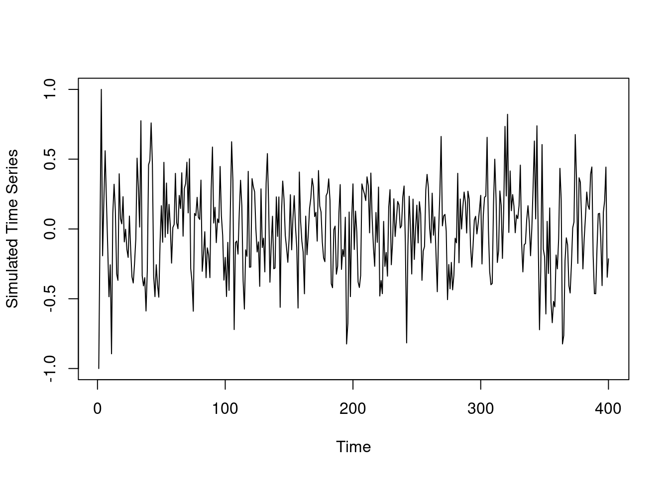
We generate some data from the three component mixture of AR(2) process.
Given $y_1=-1$ and $y_2=0$ we generate $y_3$ to $y_{3:200}$ from the following distribution:
$$
\begin{aligned}
y_i \sim 0.5\ \mathcal{N}(0.1 y_{t-1} + 0.1 y_{t-2}, 0.25) \\
+\ 0.3\ \mathcal{N}(0.4 y_{t-1} - 0.5 y_{t-2}, 0.25) \\
+\ 0.2\ \mathcal{N}(0.3 y_{t-1} + 0.5 y_{t-2}, 0.25)
\end{aligned}
$$
```{r}
#| label: fig-capstone-lsm-sim
#| fig-cap: "Simulated Time Series"
## simulate data
y=c(-1,0,1)
T.all=400

for (i in 4:T.all) {
  set.seed(i)
  U=runif(1)
  if(U<=0.5){
    y.new=rnorm(1,0.1*y[i-1]+0.1*y[i-2],0.25)
  }else if(U>0.8){
    y.new=rnorm(1,0.3*y[i-1]+0.5*y[i-2],0.25)
  }else{
    y.new=rnorm(1,0.4*y[i-1]-0.5*y[i-2],0.25)
  }
  y=c(y,y.new)
}


plot(y,type='l',xlab='Time',ylab='Simulated Time Series')
```
### Setting the Prior
We will fit a location and scale mixture of AR(2) models using 3 components. That is, $p=2$ and $K=3$. Firstly, we set up the model by choosing prior hyperparameters. We use weakly informative prior for all parameters. That is, we set :
- $a_1 = a_2 = a_3 = 1$,
- $m_0 = (0, 0)^\top$, $C_0 = 10 \times I_2$, and
- $n_0 = d_0 = 1$.
They are specified using the following code.
```{r}
#| label: lst-capstone-lsm-priors
library(MCMCpack)
library(mvtnorm)

##
p=2 ## order of AR process
K=3 ## number of mixing component
Y=matrix(y[3:200],ncol=1) ## y_{p+1:T}
Fmtx=matrix(c(y[2:199],y[1:198]),nrow=2,byrow=TRUE) ## design matrix F
n=length(Y) ## T-p


## prior hyperparameters
m0=matrix(rep(0,p),ncol=1)
C0=10*diag(p)
C0.inv=0.1*diag(p)
n0=1
d0=1
a=rep(1,K)
```
### Sampling Functions
```{r}
#| label: lst-capstone-lsm-sampling
sample_omega=function(L.cur){
  n.vec=sapply(1:K, function(k){sum(L.cur==k)})
  rdirichlet(1,a+n.vec)
}


sample_L_one=function(beta.cur,omega.cur,nu.cur,y.cur,Fmtx.cur){
  prob_k=function(k){
    beta.use=beta.cur[((k-1)*p+1):(k*p)]
    omega.cur[k]*dnorm(y.cur,mean=sum(beta.use*Fmtx.cur),sd=sqrt(nu.cur[k]))
  }
  prob.vec=sapply(1:K, prob_k)
  L.sample=sample(1:K,1,prob=prob.vec/sum(prob.vec))
  return(L.sample)
}

sample_L=function(y,x,beta.cur,omega.cur,nu.cur){
  L.new=sapply(1:n, function(j){sample_L_one(beta.cur,omega.cur,nu.cur,y.cur=y[j,],Fmtx.cur=x[,j])})
  return(L.new)
}


sample_nu=function(k,L.cur){
  idx.select=(L.cur==k)
  n.k=sum(idx.select)
  if(n.k==0){
    d.k.star=d0
    n.k.star=n0
  }else{
    y.tilde.k=Y[idx.select,]
    Fmtx.tilde.k=Fmtx[,idx.select]
    e.k=y.tilde.k-t(Fmtx.tilde.k)%*%m0
    Q.k=t(Fmtx.tilde.k)%*%C0%*%Fmtx.tilde.k+diag(n.k)
    Q.k.inv=chol2inv(chol(Q.k))
    d.k.star=d0+t(e.k)%*%Q.k.inv%*%e.k
    n.k.star=n0+n.k
  }
  1/rgamma(1,shape=n.k.star/2,rate=d.k.star/2)
}

sample_beta=function(k,L.cur,nu.cur){
  nu.use=nu.cur[k]
  idx.select=(L.cur==k)
  n.k=sum(idx.select)
  if(n.k==0){
    m.k=m0
    C.k=C0
  }else{
    y.tilde.k=Y[idx.select,]
    Fmtx.tilde.k=Fmtx[,idx.select]
    e.k=y.tilde.k-t(Fmtx.tilde.k)%*%m0
    Q.k=t(Fmtx.tilde.k)%*%C0%*%Fmtx.tilde.k+diag(n.k)
    Q.k.inv=chol2inv(chol(Q.k))
    A.k=C0%*%Fmtx.tilde.k%*%Q.k.inv
    m.k=m0+A.k%*%e.k
    C.k=C0-A.k%*%Q.k%*%t(A.k)
  }

  rmvnorm(1,m.k,nu.use*C.k)
}
```
### The Gibbs Sampler
```{r}
#| label: lst-capstone-lsm-gibbs-init
## number of iterations
nsim=20000


## store parameters


beta.mtx=matrix(0,nrow=p*K,ncol=nsim)
L.mtx=matrix(0,nrow=n,ncol=nsim)
omega.mtx=matrix(0,nrow=K,ncol=nsim)
nu.mtx=matrix(0,nrow=K,ncol=nsim)


## initial value
beta.cur=rep(0,p*K)
L.cur=rep(1,n)
omega.cur=rep(1/K,K)
nu.cur=rep(1,K)
```
Now everything has been set up, we can start to code the loop.
Note it may take a while to complete the loop.
```{r}
#| label: lst-capstone-lsm-gibbs-sampler
## Gibbs Sampler
for (i in 1:nsim) {
  set.seed(i)

  ## sample omega
  omega.cur=sample_omega(L.cur)
  omega.mtx[,i]=omega.cur

  ## sample L
  L.cur=sample_L(Y,Fmtx,beta.cur,omega.cur,nu.cur)
  L.mtx[,i]=L.cur

  ## sample nu
  nu.cur=sapply(1:K,function(k){sample_nu(k,L.cur)})
  nu.mtx[,i]=nu.cur

  ## sample beta
  beta.cur=as.vector(sapply(1:K, function(k){sample_beta(k,L.cur,nu.cur)}))
  beta.mtx[,i]=beta.cur

  ## show the numer of iterations
  if(i%%1000==0){
    print(paste("Number of iterations:",i))
  }

}
```
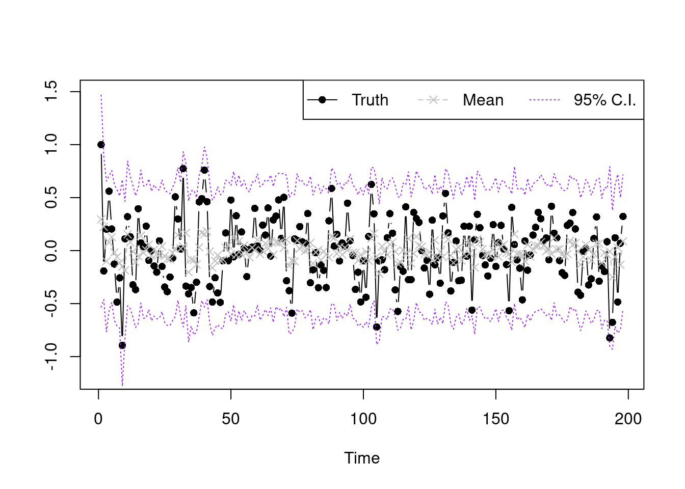
### Checking the Posterior Inference Result
Finally, we plot the posterior mean and interval estimate of the original data using the later 10000 posterior samples, which is shown below.
```{r}
#| label: fig-capstone-lsm-pred
sample.select.idx=seq(10001,20000,by=1)

post.pred.y.mix=function(idx){

  k.vec.use=L.mtx[,idx]
  beta.use=beta.mtx[,idx]
  nu.use=nu.mtx[,idx]


  get.mean=function(s){
    k.use=k.vec.use[s]
    sum(Fmtx[,s]*beta.use[((k.use-1)*p+1):(k.use*p)])
  }
  get.sd=function(s){
    k.use=k.vec.use[s]
    sqrt(nu.use[k.use])
  }
  mu.y=sapply(1:n, get.mean)
  sd.y=sapply(1:n, get.sd)
  sapply(1:length(mu.y), function(k){rnorm(1,mu.y[k],sd.y[k])})

}

y.post.pred.sample=sapply(sample.select.idx, post.pred.y.mix)


summary.vec95=function(vec){
  c(unname(quantile(vec,0.025)),mean(vec),unname(quantile(vec,0.975)))
}


summary.y=apply(y.post.pred.sample,MARGIN=1,summary.vec95)


plot(Y,type='b',xlab='Time',ylab='',pch=16,ylim=c(-1.2,1.5))
lines(summary.y[2,],type='b',col='grey',lty=2,pch=4)
lines(summary.y[1,],type='l',col='purple',lty=3)
lines(summary.y[3,],type='l',col='purple',lty=3)
legend("topright",legend=c('Truth','Mean','95% C.I.'),lty=1:3,
       col=c('black','grey','purple'),horiz = T,pch=c(16,4,NA))
```