---
date: 2024-11-01
title: "Stationarity, The ACF and the PCF"
subtitle: Time Series Analysis
description: "This lesson we will define the AR(1) process, Stationarity, ACF, PACF, differencing, smoothing"
categories:
- coursera
- notes
- bayesian statistics
- autoregressive models
- time series
keywords:
- time series
- stationarity
- strong stationarity
- weak stationarity
- lag
- autocorrelation function (ACF)
- partial autocorrelation function (PACF)
- smoothing
- trend
- seasonality
- quasi-periodicity
- differencing operator
- back shift operator
- moving average
- R code
- diff function
- filter function
---
::: {.callout-note collapse="true"}
## Learning Objectives
- [x] ~~List the goals of the course~~
- [x] ~~identify the basics of the R environment.~~
- [x] Explain **stationary** time series processes
- [x] Define **auto-correlation function** (ACF) and
- [x] Define **partial auto-correlation function** (PACF)
- [x] use R to plot the sample ACF and sample PACF of a time series
- [x] Explain the concepts of differencing and smoothing via moving averages to remove/highlight trends and seasonal components in a time series
:::
## Introduction {#sec-c4-introduction}
### Welcome to Bayesian Statistics: Time Series
- [x] Obligatory introduction to the course and the instructors.
- [Raquel Prado]() is a professor of statistics in the [Baskin School of Engineering](https://engineering.ucsc.edu/) at the University of California, Santa Cruz. She was the recipient 2022 [Zellner Medal](https://bayesian.org/project/zellner-medal/), see @BibEntry2024Sep.
### Introduction to R
- [x] [Introduction to R](https://cran.r-project.org/doc/manuals/r-release/R-intro.pdf)
## Stationarity the ACF and the PACF :movie_camera: {#sec-stationarity-acf-pacf}
Before diving into the material here is a brief overview of the notations for timer series.
::: {#tip-notation .callout-tip}
#### Notation
- $\{y_t\}$ - the time series process, where each $y_t$ is a univariate random variable and t are the time points that are equally spaced.
- $y_{1:T}$ or $y_1, y_2, \ldots, y_T$ - the observed data.
- You will see the use of ' to denote the transpose of a matrix,
- and the use of $\sim$ to denote a distribution.
- under tildes $\utilde{y}$ are used to denote estimates of the true values $y$.
- E matrix of eigenvalues
- $\Lambda = diagonal(\alpha_1, \alpha_2, \ldots , \alpha_p)$ is a diagonal matrix with the eigenvalues of $\Sigma$ on the diagonal.
- $J_p(1)$ = a p by p [Jordan form](https://en.wikipedia.org/wiki/Jordan_normal_form) matrix with 1 on the super-diagonal
also see [@prado2023time pp. 2-3]
:::
### Stationarity :movie_camera:
{#fig-slide-stationarity-1 .column-margin group="slides" width="53mm"}
\index{stationarity}
Stationarity c.f. [@prado2023time §1.2] is a fundamental concept in time series analysis.
::: {.callout-important}
## TL;DR -- Stationarity
Stationarity
: [Stationarity]{.column-margin}
: A time series is said to be stationary if its statistical properties such as mean, variance, and auto-correlation do not change over time.
- We make this definition more formal in the definitions of strong and weak stationarity below.
:::
[Stationarity is a key concept in time series analysis. A time series is said to be stationary if its statistical properties such as mean, variance, and auto-correlation do not change over time.]{.mark}
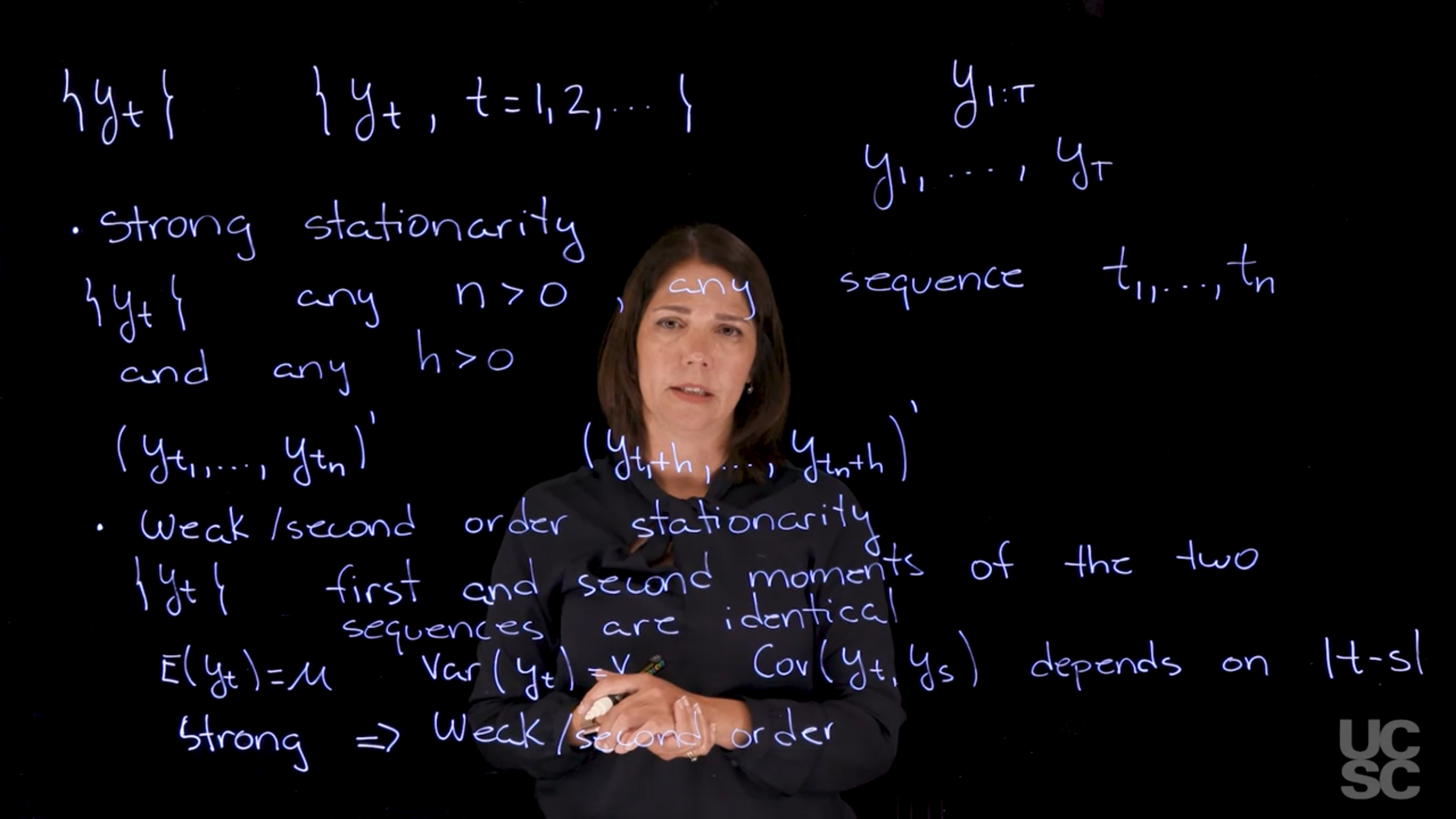
::: {#def-strong-stationarity}
## Strong Stationarity
\index{stationarity!strong}
[Strong Stationarity]{.column-margin} Let $y_t$ be a time series. We say that $y_t$ is *stationary* if the following conditions hold:
Let $\{y_t\} \quad \forall n>0$ be a time series and $h > 0$ be a lag. If for any subsequence the distribution of $y_t, y_{t+1}, \ldots, y_{t+n}$ is the same as the distribution of $y_{t+h}, y_{t+h+1}, \ldots, y_{t+h+n}$ we call the series strongly stationary.
:::
As it's difficult to verify strong stationarity in practice, we will often use the following weaker notion of stationarity.
::: {#def-weak-stationarity}
## Weak Stationarity
\index{stationarity!weak }
[Weak Stationarity]{.column-margin} [Second-order Stationarity]{.column-margin} The mean, variance, and auto-covariance are constant over time.
$$
\begin{aligned}
\mathbb{E}[y_t] &= \mu \quad \forall t \\
\mathbb{V}ar[y_t] &= \nu =\sigma^2 \quad \forall t \\
\mathbb{C}ov[y_t , y_s ] &= γ(t − s)
\end{aligned}
$$ {#eq-weak-stationarity}
:::
- Strong stationarity $\implies$ Weak stationarity, but
- The converse is not true.
- In this course when we deal with a Gaussian process, our typical use case, they are equivalent!
::: {.callout-note collapse="true"}
## Video Transcript
{{< include transcripts/c4/01_week-1-introduction-to-time-series-and-the-ar-1-process/02_stationarity-the-acf-and-the-pacf/01_stationarity.en.txt >}}
:::
Going over the transcript I have a couple of points.
Prado mentions a couple of concepts like a moving average process and a Gaussian process in this lesson but does not define them in this course. In fact neither are defined in the specialization. While a Gaussian process is a non-parametric model and is a bit more advanced a moving average process is part of the ARMA family of models and we do delve into these in both this and the next course of the specialization.
::: {.callout-caution}
## Check your understanding
Q. Can you explain with an example when a time series is weakly stationary but not strongly stationary?
:::
### The auto-correlation function ACF :movie_camera: {#sec-acf}
{#fig-slide-afc-1 .column-margin group="slides" width="53mm"}
\index{auto correlation function}
\index{ACF|\see {auto correlation function}}
[The auto correlation is simply how correlated a time series is with itself at different lags]{.mark}.
- Correlation in general is defined in terms of covariance of two variables.
- The covariance is a measure of the joint variability of two random variables.
::: {.callout-important}
Recall that the Covariance between two random variables $y_t$ and $y_s$ is defined as:
$$
\begin{aligned}
\mathbb{C}ov[y_t, y_s] &= \mathbb{E}[(y_t-\mathbb{E}[y_t])(y_s-\mathbb{E}[y_s])] \\
&= \mathbb{E}[(y_t-\mu_t)(y_s-\mu_s)] \\
&= E[y_t y_s] - \mu_t \times \mu_s
\end{aligned} \qquad
$$ {#eq-covariance}
We get the second line by substituting
$\mu_t = \mathbb{E}(y_t)$
and
$\mu_s = \mathbb{E}(y_s)$
using the definition of the mean of a RV.
the third line is by multiplying out and using the linearity of the expectation operator.
:::
::: {#tip-acf .callout-tip }
### AFC notation {#sec-afc-notation}
We will frequently use the notation $\gamma(h)$ to denote the **autocovariance** for a lag $h$ i.e. between $y_t$ and $y_{t+h}$
$$
\gamma(h) = \mathbb{C}ov[y_t, y_{t+h}] \qquad
$$ {#eq-autocovariance}
:::
When the time series is stationary, then the covariance only depends on the lag
$h = \|t-s\|$ and we can write the covariance as $\gamma(h)$.
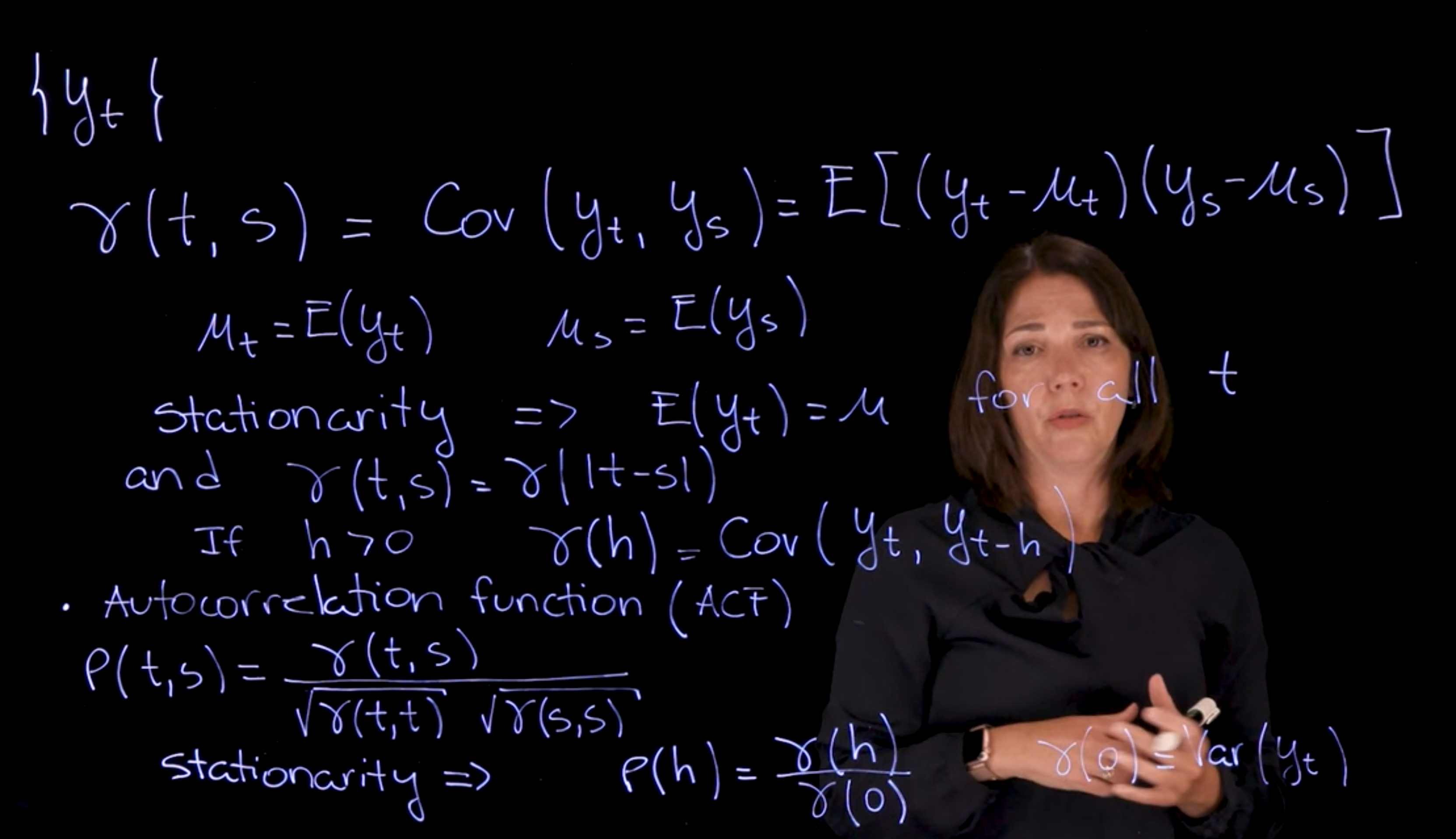
Let $\{y_t\}$ be a time series. Recall that the covariance between two random variables $y_t$ and $y_s$ is defined as:
$$
\gamma(t,s)=\mathbb{C}ov[y_t, y_s] = \mathbb{E}[(y_t-\mu_t)(y_s-\mu_s)] \qquad
$$ {#eq-covariance}
where $\mu_t = \mathbb{E}(y_t)$ and $\mu_s = \mathbb{E}(y_s)$ are the means of $y_t$ and $y_s$ respectively.
$$
\mu_t = \mathbb{E}(y_t) \qquad \mu_s = \mathbb{E}(y_s)
$$ {#eq-mean}
$$
\text{Stationarity} \implies \mathbb{E}[y_t] = \mu \quad \forall t \qquad \therefore \quad \gamma(t,s)=\gamma(|t-s|)
$$
If $h>0 \qquad \gamma(h)=\mathbb{C}ov[y_t,y_{t-h}]$
::: {.callout-important}
### Autocorrelation Function (AFC) {#sec-autocorrelation-function}
[auto-correlation AFC]{.column-margin}
$$
\rho(t,s) = \frac{\gamma(t,s)}{\sqrt{\gamma(t,t)\gamma(s,s)}}
$$ {#eq-autocorrelation}
:::
$$
\text{Stationarity} \implies \rho(h)=\frac{\gamma(h)}{\gamma(o)} \qquad \gamma(0)=Var(y_t)
$$
{#fig-slide-afc-2 .column-margin group="slides" width="53mm"}
$$
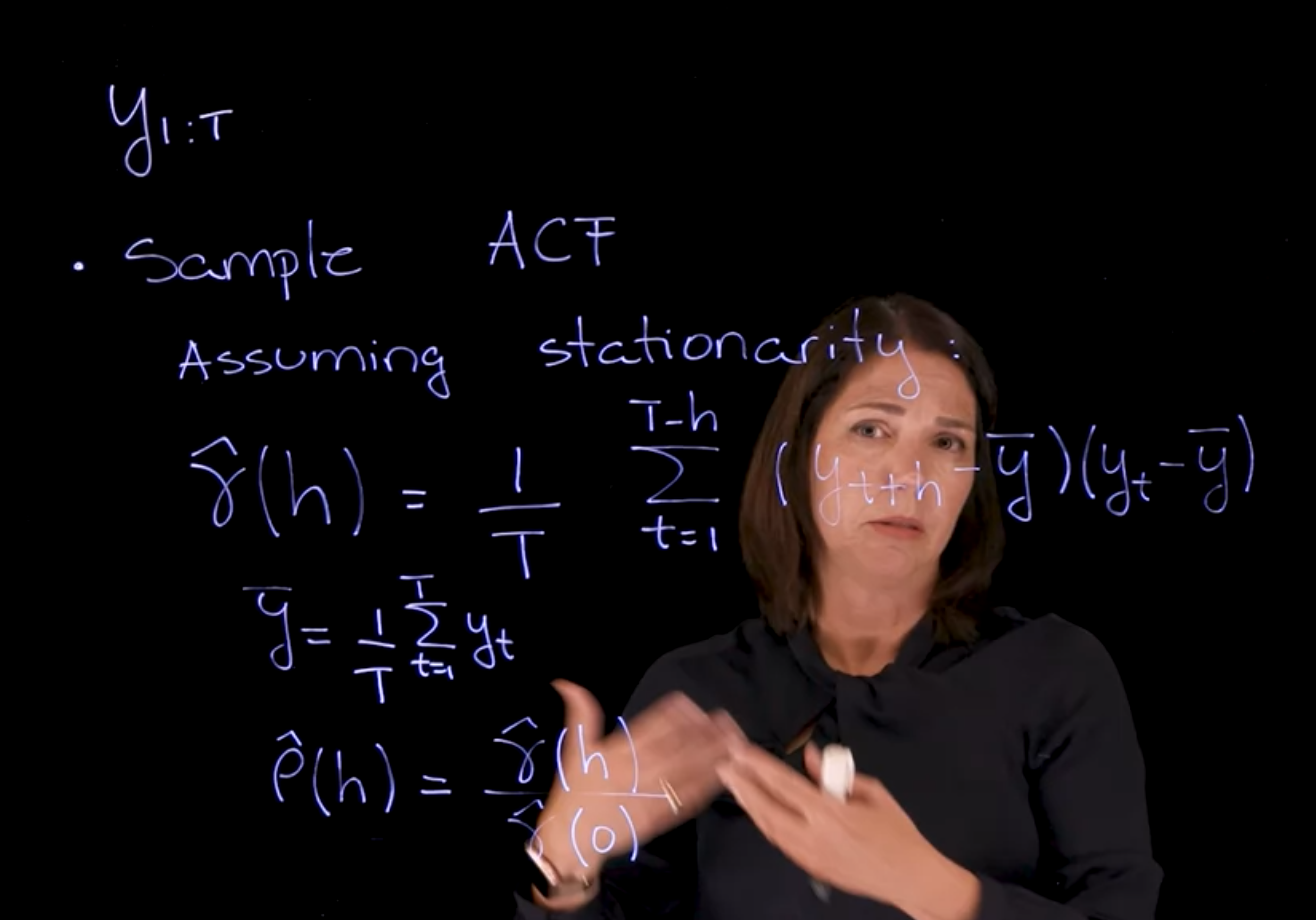
y_{1:T}
$$ {#eq-sub-sequence}
::: {.callout-important}
### The sample AFC {#sec-sample-acf}
$$
\hat\gamma(h)= \frac{1}{T} \sum_{t=1}^{T-h}(y_{t+h}-\bar y )(y_t-\hat y)
$$ {#eq-sample-auto-covariance-function}
where $\bar y$ is the sample mean of the time series $y_{1:T}$, and $\hat y$ is the sample mean of the time series $y_{1:T-h}$.
:::
$$
\bar y = \frac{1}{T} \sum_{t=1}^{T}y_t
$$ {#eq-sample-mean}
$$
\hat \rho = \frac{\hat\gamma(h)}{\hat\gamma(o)}
$$ {#eq-sample-auto-correlation-function}
### The partial auto-correlation function PACF :spiral_notepad: {#sec-pacf-reading}
::: {#def-pacf }
## Partial Auto-correlation Function (PACF)
Let ${y_t}$ be a zero-mean stationary process, and let
$$
\hat{y}_t^{h-1} = \beta_1 y_{t-1} + \beta_2 y_{t-2} + \ldots + \beta_{h-1} y_{t-(h-1)}
$$ {#eq-best-linear-predictor}
be the best linear predictor of $y_t$ based on the previous $h − 1$ values $\{y_{t−1}, \ldots , y_{t−h+1}\}$. The best linear predictor of $y_t$ based on the previous $h − 1$ values of the process is the linear predictor that minimizes
$$
\mathbb{E}[(y_t − \hat{y}_y^{h-1})^2]
$$ {#eq-best-linear-predictor-minimization}
The partial autocorrelation of this process at lag h, denoted by $\phi(h, h)$ is defined as: [partial auto-correlation PAFC]{.column-margin}
$$
\phi(h, h) = Corr(y_{t+h} − \hat{y}_{t+h}^{h-1}, y_t − \hat{y}_t^{h-1})
$$ {#eq-partial-auto-correlation}
for $h \ge 2$ and $\phi(1, 1) = Corr(y_{t+1}, y_{t}) = \rho(1)$.
:::
The partial autocorrelation function can also be computed via the Durbin-Levinson recursion for stationary processes as $\phi(0, 0) = 0$,
$$
\phi(n, n) = \frac{\rho(n) − \sum_{h=1}^{n-1} \phi(n − 1, h)\rho(n − h)}{1- \sum_{h=1}^{n-1}\phi(n − 1, h)\rho(h)}
$$ {#eq-durbin-levinson}
for $n \ge 1$, and
$$
\phi(n, h) = \phi(n − 1, h) − \phi(n, n)\phi(n − 1, n − h),
$$ {#eq-durbin-levinson-2}
for $n \ge 2$, and $h = 1, \ldots , (n − 1)$.
Note that the sample PACF can be obtained by substituting the sample autocorrelations and the sample auto-covariances in the Durbin-Levinson recursion.
::: {.callout-note collapse="true"}
## Video Transcript
{{< include transcripts/c4/01_week-1-introduction-to-time-series-and-the-ar-1-process/02_stationarity-the-acf-and-the-pacf/02_the-autocorrelation-function-acf.en.txt >}}
:::
## Differencing and smoothing :spiral_notepad: {#sec-differencing-and-smoothing}
\index{differencing}
\index{smoothing}
Differencing and smoothing are techniques used to remove trends and seasonality in time series data. They are covered in the [@prado2023time §1.4].
Many synthetic time series models are built under the assumption of stationarity. However, in the real world time series data often present non-stationary features such as **trends** or **seasonality**. These features render such a time series non-stationary, and therefore, not suitable for analysis using the tools and methods we have discussed so far. However practitioners can use techniques for detrending, deseasonalizing and smoothing that when applied to such observed data transforms it into a new time series that is consistent with the stationarity assumption.
We briefly discuss two methods that are commonly used in practice for detrending and smoothing.
### Differencing
[Differencing, is a method which removes the trend from a time series data]{.mark}. The first difference of a time series is defined in terms of the difference operator, denoted as $D$, that produces the transformation [differencing operator $D$]{.column-margin}
$$
Dy_t \doteqdot y_t - y_{t-1}
$$ {#eq-first-difference-operator-definition}
Higher order differences are obtained by successively applying the operator $D$. For example,
$$
D^2y_t = D(Dy_t) = D(y_t - y_{t-1}) = y_t - 2y_{t-1} + y_{t-2}
$$ {#eq-higher-order-difference-operator-definition}
Differencing can also be written in terms of the so called back-shift operator $B$, with [back-shift operator $B$]{.column-margin}
$$
By_t \doteqdot y_{t-1},
$$ {#eq-backshift-operator-definition}
so that
$$
Dy_t \doteqdot (1 - B) y_t
$$ {#eq-first-difference-operator-via-back-shift-definition}
and
$$
D^dy_t \doteqdot (1 - B)^d y_t.
$$ {#eq-higher-order-difference-operator-definition}
this notation lets us write the differences in by referencing items backwards in time, which is often more intuitive and also useful, for example, when we will want to write the differencing operator in terms of a polynomial.
### Smoothing
\index{smoothing}
\index{moving average}
[Moving averages, which is commonly used to "smooth" a time series by removing certain features (e.g., seasonality) to highlight other features]{.mark} (e.g., trends).
[A moving average is a weighted average of the time series around a particular time]{.mark} $t$. In general, if we have data $y_{1:T}$, we could obtain a new time series such that [moving average]{.column-margin}
$$
z_t = \sum_{j=-q}^{p} w_j y_{t+j} \qquad
$$ {#eq-moving-average}
for $t = (q + 1) : (T − p)$, with weights $w_j \ge 0$ and $\sum^p_{j=−q} w_j = 1$
We will frequently work with *moving averages* for which
$$
p = q \qquad \text{(centered)}
$$
and
$$
w_j = w_{−j} \forall j \text{(symmetric)}
$$
Assume we have periodic data with period $d$. Then, symmetric and centered moving averages can be used to remove such periodicity as follows:
- If $d = 2q$ :
$$
z_t = \frac{1}{d} \left(\frac{1}{2} y_{t−q} + y_{t−q+1} + \ldots + y_{t+q−1} + \frac{1}{2} y_{t+q}\right )
$$ {#eq-even-seasonal-moving-average}
- if $d = 2q + 1$ :
$$
z_t = \frac{1}{d} \left( y_{t−q} + y_{t−q+1} + \ldots + y_{t+q−1} + y_{t+q}\right )
$$ {#eq-odd-seasonal-moving-average}
::: {#exm-seasonal-moving-average}
### Seasonal Moving Average
To remove seasonality in monthly data (i.e., seasonality with a period of d = 12 months), we use a moving average with $p = q = 6$, $a_6 = a_{−6} = 1/24$, and $a_j = a_{−j} = 1/12$ for $j = 0, \ldots , 5$ , resulting in:
$$
z_t = \frac{1}{24} y_{t−6} + \frac{1}{12}y_{t−5} + \ldots + \frac{1}{12}y_{t+5} + \frac{1}{24}y_{t+6}
$$ {#eq-seasonal-moving-average}
:::
## ACF PACF Differencing and Smoothing Examples :movie_camera: {#sec-differencing-and-smoothing-examples}
This video walks us through the code snippets in @fig-moving-averages-and-differencing and @fig-white-noise-simulation below and provides examples of how to compute the ACF and PACF of a time series, how to use differencing to remove trends, and how to use moving averages to remove seasonality.
- We begin by simulating data using the code in @sec-white-noise-simulation
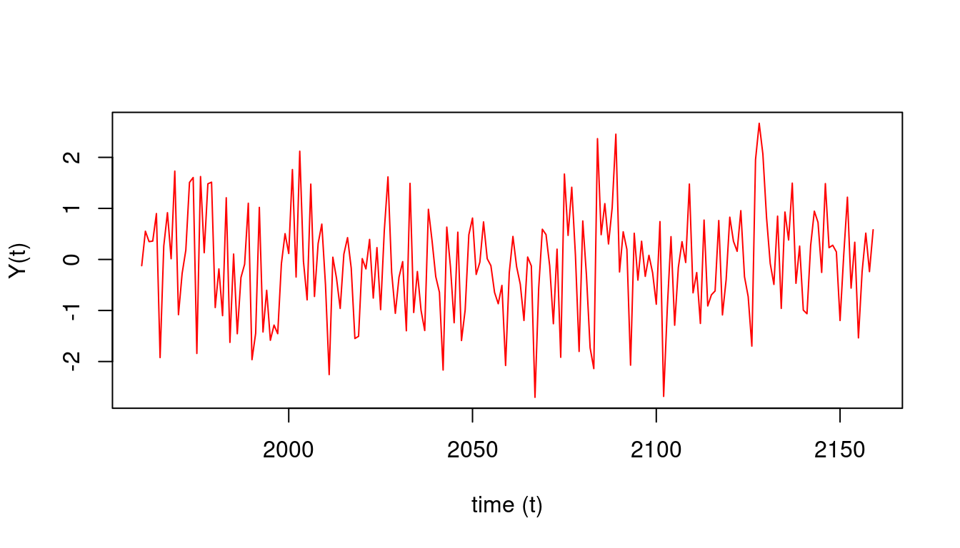
- We simulates white noise data using the `rnorm(1:2000,mean=0,sd=1)` function in `R`
- We plot the white noise data which we can see lacks a temporal structure.
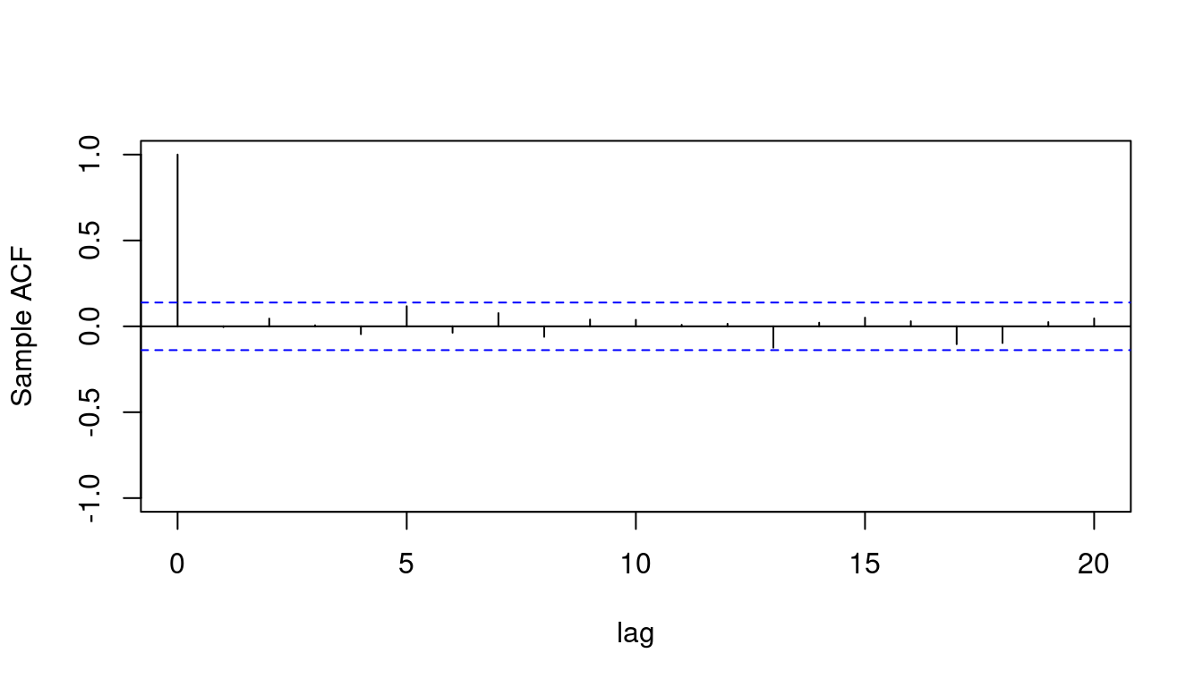
- We plot the *ACF* using the `acf` function in `R`:
- we specify the number of lags using the `lag.max=20`
- we shows a confidence interval for the ACF values
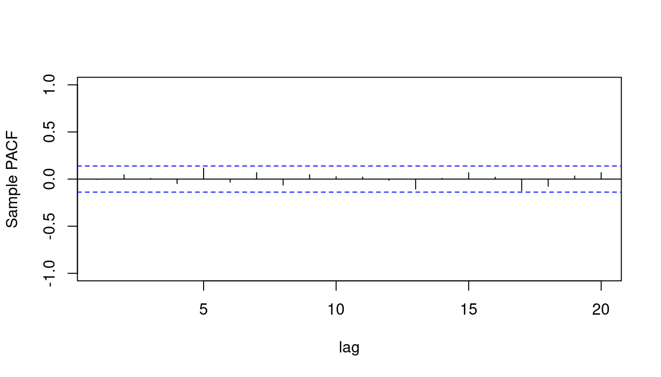
- We plot the *PACF* using the `pacf` function in `R`
- Next we define some time series objects in `R` using the `ts` function
- we define and plot monthly data starting in January 1960
- we define and plot yearly data with one observation per year starting in 1960
- we define and plot yearly data with four observations per year starting in 1960
- We move on to smoothing and differencing in @sec-differencing-and-smoothing
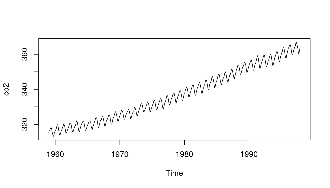
- We load the CO2 dataset in `R` and plot it
- we plot the *ACF* and *PACF* of the CO2 dataset
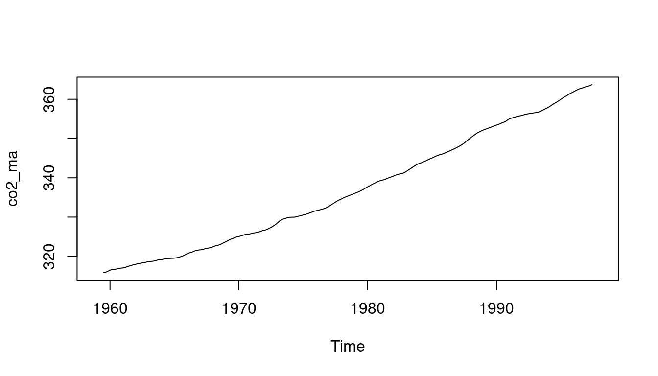
- we use the `filter` function in `R` to remove the seasonal component of the CO2 dataset we plot the resulting time series highlighting the trend.
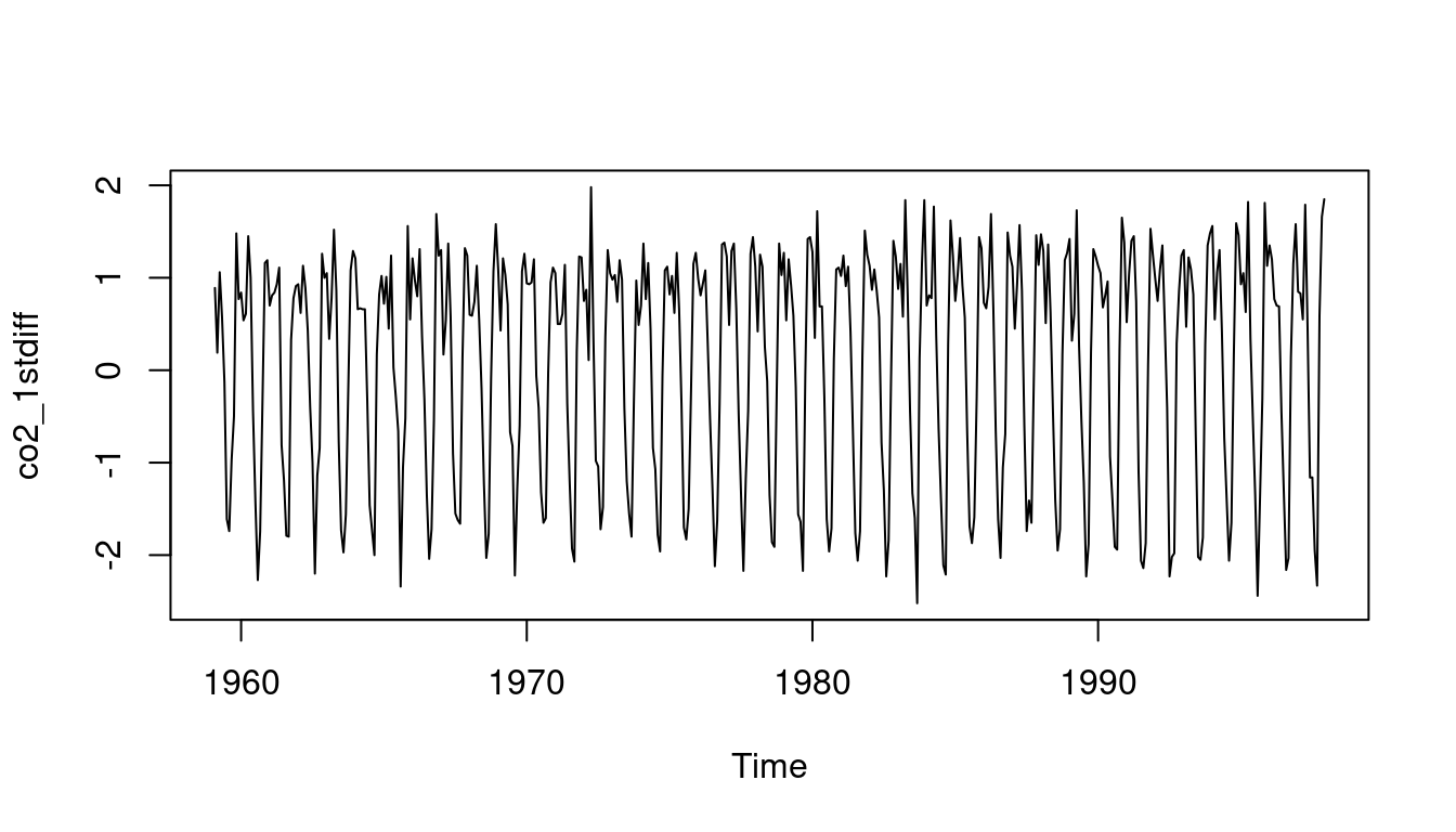
- To remove the trend we use the `diff` function in `R` to take the first and second differences of the CO2 dataset
- the `diff` function takes a parameter `differences` which specifies the number of differences to take
- we plot the resulting time series after taking the first and second differences
- the *ACF* and *PACF* of the resulting time series are plotted, they look different, in that they no longer have the slow decay characteristic of time series with a trend.
::: {.callout-note collapse="true"}
## Video Transcript
{{< include transcripts/c4/01_week-1-introduction-to-time-series-and-the-ar-1-process/02_stationarity-the-acf-and-the-pacf/05_acf-pacf-differencing-and-smoothing-examples.en.txt >}}
:::
## Code for Differencing and filtering via moving averages :spiral_notepad: $\mathcal{R}$ {#sec-differencing-and-smoothing-reading}
\index{dataset!CO2}
\index{differencing}
\index{smoothing}
\index{moving average}
\index{filtering}
```{r}
#| label: fig-moving-averages-and-differencing
#| lst-label: lst-moving-averages-and-differencing
#| fig-cap: "Differencing and filtering via moving averages"
#| fig-subcap:
#| - "the original data"
#| - "the first difference (TS - trend), highlightes the seasonality"
#| - "the moving averages (TS - seasonality), highlights the trend"
#| layout-nrows: 3
#| fig.height: 4
#| fig.width: 7
data(co2) # <1>
co2_1stdiff = diff(co2,differences=1) # <2>
co2_ma = filter(co2,filter=c(1/24,rep(1/12,11),1/24),sides=2) # <3>
#par(mfrow = c(3,1), mar = c(3, 4, 2, 1), cex.lab=1.2, cex.main=1.2)
plot(co2) # <4>
plot(co2_1stdiff) # <5>
plot(co2_ma) # <6>
```
1. Load the CO2 dataset in R
2. Take first differences to remove the trend
3. Filter via moving averages to remove the seasonality
4. plot the original data
5. plot the first differences (removes trend, highlights seasonality)
6. plot the filtered series via moving averages (removes the seasonality, highlights the trend)
## Code: Simulate data from a white noise process :spiral_notepad: $\mathcal{R}$ {#sec-white-noise-simulation}
\index{white noise}
\index{process!white noise}
\index{process!Wiener}
\index{Brownian motion}
```{r}
#| label: fig-white-noise-simulation
#| lst-label: lst-white-noise-simulation
#| fig-cap:
#| - "Simulate white noise data"
#| fig-subcap:
#| - "Simulate data with no temporal structure (white noise)"
#| - "Sample AFC"
#| - "Sample PACF"
#| fig.height: 4
#| fig.width: 7
#| layout-nrows: 2
set.seed(2021)
T=200
t =1:T
y_white_noise=rnorm(T, mean=0, sd=1)
yt=ts(y_white_noise, start=c(1960), frequency=1) # <1>
#par(mfrow = c(3, 1), mar = c(3, 4, 2, 1), cex.lab = 1.3, cex.main = 1.3)
plot(yt, type = 'l', col='red', # <2>
xlab = 'time (t)',
ylab = "Y(t)") # <2>
acf(yt, # <3>
lag.max = 20,
xlab = "lag",
ylab = "Sample ACF",
ylim=c(-1,1),main="") # <3>
pacf(yt, lag.max = 20, # <4>
xlab = "lag", ylab = "Sample PACF", # <4>
ylim=c(-1,1),main="") # <4>
```
1. Define a time series object in R - Assume the data correspond to annual observations starting in January 1960
2. Plot the simulated time series,
3. Plot the sample ACF
4. Plot the sample PACF