3.1 Conditional Probability
\mathbb{P}r(A \mid B)=\frac{\mathbb{P}r(A \cap B)}{\mathbb{P}r(B)} \tag{3.1}
independence
\mathbb{P}r(A \mid B) = \mathbb{P}r(A) \implies \mathbb{P}r(A \cap B) = \mathbb{P}r(A)\mathbb{P}r(B) \tag{3.2}
3.1.1 Conditional Probability Example - Female CS Student
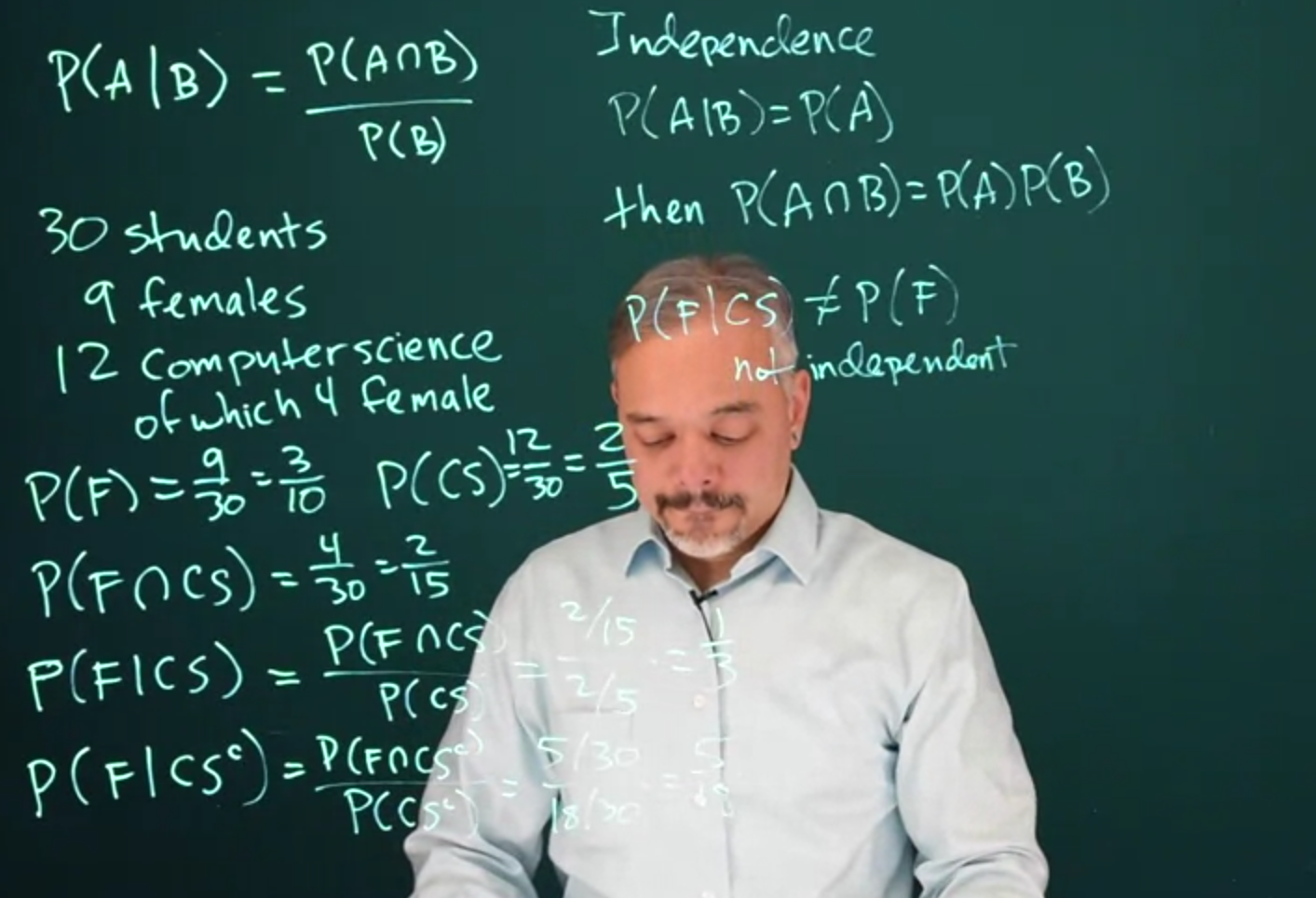
Suppose there are 30 students, 9 of whom are female. Of the 30 students, 12 are computer science majors. 4 of those 12 computer science majors are female. We want to estimate what is the probability of a student being female given that she is a computer science major We start by writing the above in the language of probability by converting frequencies to probabilities. We start with the marginal. First, the probability of a student being female from the data given above.
\mathbb{P}r(\text{Female}) = \frac{9}{30} = \frac{3}{10}
Next, we estimate the probability of a student being a computer science major again just using the data given above.
\mathbb{P}r(CS) = \frac{12}{30} = \frac{2}{5}
Next, we can estimate the joint probability, i.e. the probability of being female and being a CS major. Again we have been given the numbers in the data above.
\mathbb{P}r(F\cap CS) = \frac{4}{30} = \frac{2}{15}
Finally, we can use the definition of conditional probability and substitute the above
\mathbb{P}r(F \mid CS) = \frac{\mathbb{P}r(F \cap CS)}{\mathbb{P}r(CS)} = \frac{2/15}{2/5} = \frac{1}{3} \tag{3.3}
An intuitive way to think about a conditional probability is that we’re looking at a sub-segment of the original population, and asking a probability question within that segment
\mathbb{P}r(F \mid CS^c) = \frac{\mathbb{P}r(F\cap CS^c)}{ \mathbb{P}r (CS^c)} = \frac{5/30}{18/30} = \frac{5}{18} \tag{3.4}
The concept of independence is when one event does not depend on another.
A \perp \!\!\! \perp B \iff \mathbb{P}r(A \mid B) = \mathbb{P}r(A)
It doesn’t matter that B occurred.
If two events are independent then the following is true:
A \perp \!\!\! \perp B \iff \mathbb{P}r(A\cap B) = \mathbb{P}r(A)\mathbb{P}r(B) \tag{3.5}
This can be derived from the conditional probability equation.
3.1.2 Inverting Conditional Probabilities
If we don’t know \mathbb{P}r(A \mid B) but we do know the inverse probability \mathbb{P}r(B \mid A) is. We can then rewrite \mathbb{P}r(A \mid B) in terms of \mathbb{P}r(B \mid A)
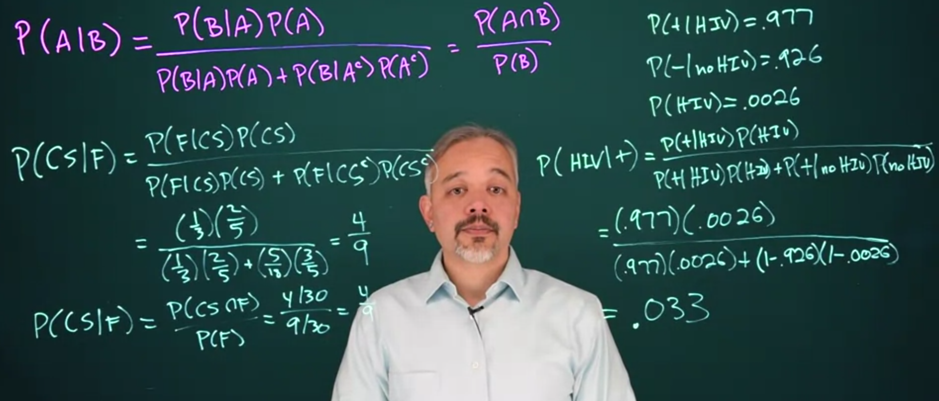
\mathbb{P}r(A \mid B) = \frac{\mathbb{P}r(B \mid A)\mathbb{P}r(A)}{\mathbb{P}r(B \mid A)\mathbb{P}r(A) + \mathbb{P}r(B \mid A^c)\mathbb{P}r(A^c)} \tag{3.6}
3.1.3 Conditional Probability Example - ELISA HIV test
Let’s look at an example of an early test for HIV antibodies known as:
- the ELISA test.
- The test has a true positive rate of 0.977.
- It has a true negative rate of 0.926.
- The incidence of HIV in North America is .0026.
Now we want to know the probability of an individual having the disease given that they tested positive \mathbb{P}r(\text{HIV} \mid +).
This is the inverse probability of the true positive, so we will need to use Bayes’ theorem.
We start by encoding the above using mathematical notation, so we know what to substitute into Bayes’ theorem.
The true positive rate is:
\mathbb{P}r(+ \mid \text{HIV}) = 0.977
The true negative rate is:
\mathbb{P}r(- \mid \text{HIV}) = 0.926
The false positive rate is: \mathbb{P}r(- \mid \text{NO HIV}) = 0.926
The probability of someone in North America having this disease was
\mathbb{P}r(HIV) = .0026
what we want is: \mathbb{P}r(\text{HIV} \mid +)
\begin{aligned} \mathbb{P}r(\text{HIV} \mid +) &= \frac{\mathbb{P}r(+ \mid \text{HIV})\mathbb{P}r(\text{HIV})}{\mathbb{P}r(+ \mid \text{HIV})\mathbb{P}r(\text{HIV}) + \mathbb{P}r(+ \mid \text{NO HIV})\mathbb{P}r(\text{NO HIV})} \\ &= \frac{(.977)(.0026)}{(.977)(.0026) + (1-.977)(1-.0026)} \\ &= 0.033 \end{aligned} \tag{3.7}
- This is a bit of a surprise
- although the test has 90% + true and false accuracy
- taking it once is only valid 3% of the time. How is this possible?
What happens in Bayes law is that we are updating probabilities. And since we started with such a low probability of .0026, Bayesian updating only brings it up to 0.03.
\begin{aligned} \mathbb{P}r(A \mid B) = \frac{\mathbb{P}r(B \mid A_1){(A_1)}}{\sum_{i=1}^{n}{\mathbb{P}r(B \mid A_i)}\mathbb{P}r(A_i)} \end{aligned} \tag{3.8}
Note in (McElreath 2015) the author, discusses how this and similar concepts can be presented in a fashion that seems less surprisingly to the lay person. He suggests that we can think of the test as a filter that filters out most of the people who do not have the disease, but it is not perfect.
3.2 Bayes’ theorem 🎥
Here are a few formulations of Bayes’ theorem. We denote H for our hypothesis and E as our evidence i.e. the data!
We start by using the definition of conditional probability:
\mathbb{P}r(A \mid B) = \frac{ \mathbb{P}r(A \cap B)}{\mathbb{P}r(B)} \quad \text{(conditional probability)}
\begin{aligned} {\color{orange} \overbrace{\color{orange} \mathbb{P}r(H|E)}^{\text{Posterior}}} &= \frac{ {\color{pink} \overbrace{\color{pink} \mathbb{P}r(H \cap E)}^{\text{Joint}}} } { {\color{green} \underbrace{{\color{green} \mathbb{P}r(\text{E})}}_{\text{Marginal Evidence}}} } \\ &= \frac{ {\color{red} \overbrace{\color{red} \mathbb{P}r (\text{H})}^{\text{Prior}}} \cdot {\color{blue} \overbrace{\color{blue} \mathbb{P}r (E \mid H)}^{\text{Likelihood}}} } { {\color{green} \underbrace{{\color{green} \mathbb{P}r(E)}}_{\text{Marginal Evidence}}} } \\ &= \frac{ {\color{red} \overbrace{\color{red} \mathbb{P}r (H)}^{\text{Prior}}} \cdot {\color{blue} \overbrace{\color{blue} \mathbb{P}r (E \mid H)}^{\text{Likelihood}}} }{ {\color{green} \underbrace{\color{green} \mathbb{P}r(E \mid H) \mathbb{P}r(H) + \mathbb{P}r(E \mid H^c) \mathbb{P}r(H^c) }_{\text{Marginal Evidence}}}} \end{aligned}
- where:
- H is the hypothesis we are testing.
- E is the evidence or data we have observed.
For the last step we used the law of total probability to expand the denominator using a partition of the sample space into two mutually exclusive events H and H^c (the complement of H).
Note: though that classical Hypothesis testing is flawed in the sense that we don’t usually get to pose Hypotheses in a way that is Mutually Exclusive as stated above. We typically have a null hypothesis that posits that there is no effect (i.i.e. the intervention has had no effect) which we wish to reject in lue of the alternative hypothesis that posits that there is an effect (i.e. the intervention has had an effect). This are mutually exclusive statements.
However we usually formulate our our hypothesis more narrowly, lets consider hypotension treatments
- H_0 - nothing happened despite the intervention,
- H_1 - the placebo had minimal effect.
- H_2 - Drug A reduces blood pressure more than the placebo,
- H_3 - Drug B reduces blood pressure more than Drug A,
- H_4 - Vegan diet reduces blood pressure,
- H_5 - Weight loss diet reduces blood pressure,
- H_6 - Aerobics exercise reduces blood pressure,
- H_7 - Anaerobic exercise reduces blood pressure,
Yet there are many more hypotheses we can test, including combinations of these hypotheses. However we may not be able to state them as mutually exclusive events and so we may not be able to use Bayes’ theorem as stated above.
We can extend Bayes theorem to cases with multiple mutually exclusive events:
if H_1 \ldots H_n are mutually exclusive events that sum to 1:
\begin{aligned} \mathbb{P}r(H_1 \mid E) & = \frac{\mathbb{P}r(E \mid H)\mathbb{P}r(H_1)}{\mathbb{P}r(E \mid H_1)\mathbb{P}r(H_1) +\ldots + \mathbb{P}r(E \mid H_n)\mathbb{P}r(H_N)} \\ & = \frac{\mathbb{P}r(E \mid H)\mathbb{P}r(H_1)}{\sum_{i=1}^{N} \mathbb{P}r(E \mid H_i)\mathbb{P}r(H_i)} \end{aligned}
where we used the law of total probability in the denominator
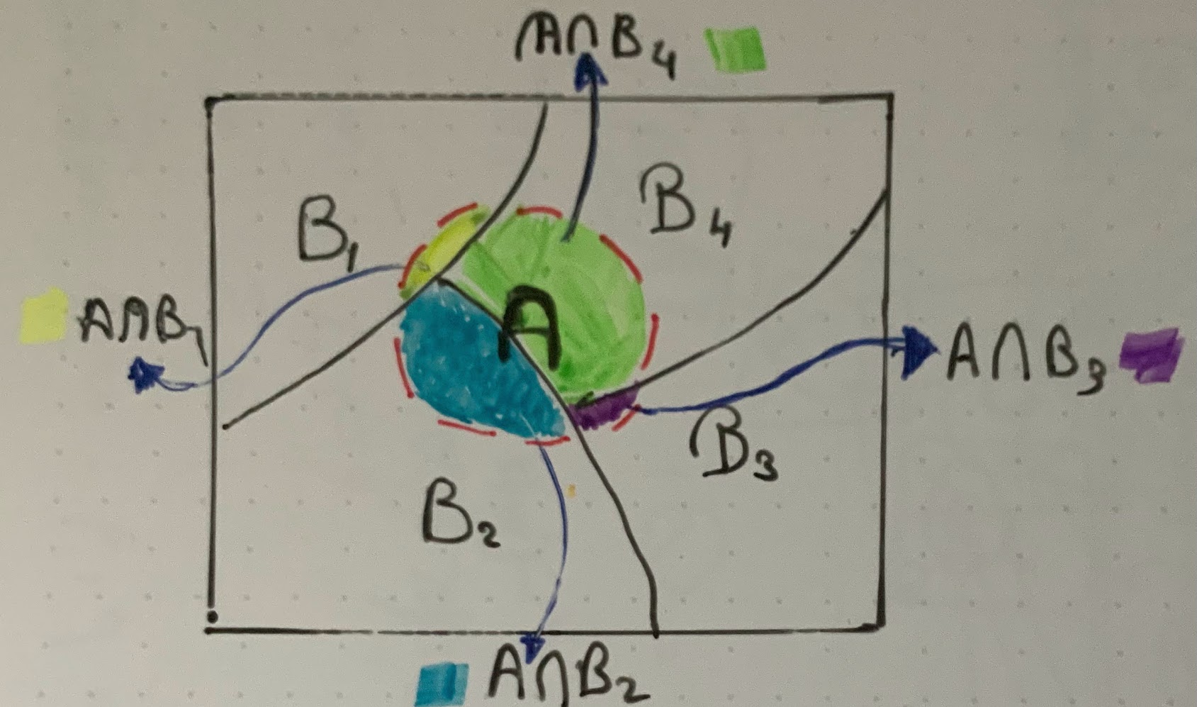
if \{B_i\} is a finite or countably finite partition of a sample space then
\mathbb{P}r(A) = {\sum_{i=1}^{N} \mathbb{P}r(A \cup B_i)}= {\sum_{i=1}^{N} \mathbb{P}r(A \mid B_i)\mathbb{P}r(B_i)}
{\color{orange} \mathbb{P}r (\text{H} \mid \text{E})} = \frac {{\color{red} \mathbb{P}r(\text{H})} \times {\color{blue}\mathbb{P}r(\text{E} \mid \text{H})}} {\color{gray} {\mathbb{P}r(\text{E})}}
{\color{orange} \overbrace{\color{orange} \mathbb{P}r (\text{Unknown} \mid \text{Data})}^{\text{Posterior}}} = \frac {{\color{red} \overbrace{\color{red} \mathbb{P}r (\text{Unknown})}^{\text{Prior}}} \times {\color{blue} \overbrace{\color{blue} \mathbb{P}r (\text{Data} \mid \text{Unknown})}^{\text{Likelihood}}}} {{\color{green} \underbrace{{\color{green} \mathbb{P}r(\text{E})}}_{\text{Average likelihood}}}}
The following is a video explaining Bayes law.
3.3 Bayes’ Theorem for continuous distributions
When dealing with a continuous random variable \theta, we can write the conditional density for \theta given y as:
f(\theta \mid y) =\frac{f(y\mid\theta)f(\theta)}{\int f(y\mid\theta) f(\theta) d\theta } \tag{3.9}
This expression does the same thing that the versions of Bayes’ theorem from Lesson 2 do. Because \theta is continuous, we integrate over all possible values of \theta in the denominator rather than take the sum over these values. The continuous version of Bayes’ theorem will play a central role from Lesson 5 on.
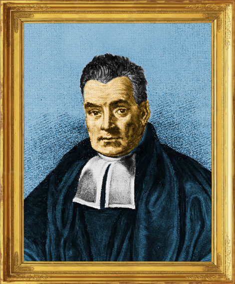
Bayes Rule is due to Thomas Bayes (1701-1761) who was an English statistician, philosopher and Presbyterian minister. Although Bayes never published what would become his most famous accomplishment; his notes were edited and published posthumously by Richard Price.