---
date: 2024-10-23
title: "Homework Bayesian analysis of an EEG dataset using an AR($p$) - M1L2HW2"
subtitle: Time Series Analysis
description: "This lesson we will define the AR(1) process, Stationarity, ACF, PACF, differencing, smoothing"
categories:
- Bayesian Statistics
keywords:
- time series
- stationarity
- strong stationarity
- weak stationarity
- lag
- autocorrelation function (ACF)
- partial autocorrelation function (PACF)
- smoothing
- trend
- seasonality
- differencing operator
- back shift operator
- moving average
---
::::: {.content-visible unless-profile="HC"}
::: {.callout-caution}
Section omitted to comply with the Honor Code
:::
:::::
::::: {.content-hidden unless-profile="HC"}
:::::
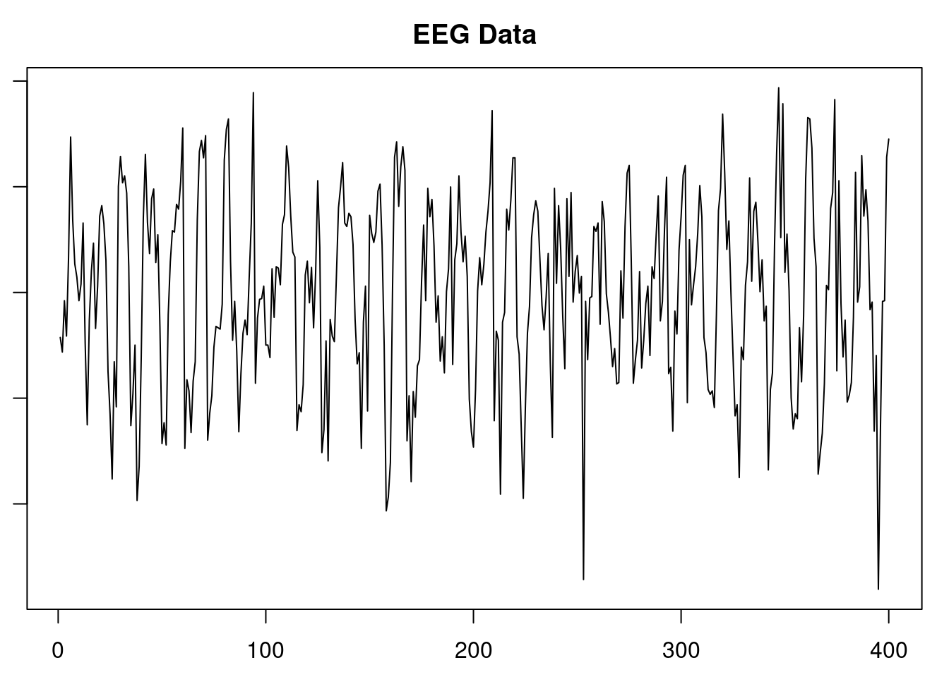
\index{dataset,EEG}
```{r}
#| label: lbl-load-eeg-data
set.seed(2021)
# Load the EEG dataset
yt=scan('data/eeg.txt')

par(mar = c(2.5, 1, 2.5, 1))

#png("eeg_plot.png", width = 800, height = 600)  # Open PNG device
# plot and save image to file()
plot(yt, type = "l", main = "EEG Data", xlab = "Index", ylab = "eeg")
# Save the plot as an image
#dev.off()  # Close the PNG device
```
convert to AR(8) process
```{r}
#| label: lbl-eeg-ar8
set.seed(2021)
yt=scan('data/eeg.txt')
T=length(yt) # length of the time series
p=8

y=rev(yt[(p+1):T]) # response
X=t(matrix(yt[rev(rep((1:p),T-p)+rep((0:(T-p-1)),rep(p,T-p)))],p,T-p));
XtX=t(X)%*%X
XtX_inv=solve(XtX)
phi_MLE=XtX_inv%*%t(X)%*%y # MLE for phi
s2=sum((y - X%*%phi_MLE)^2)/(length(y) - p) #unbiased estimate for v

cat("\n MLE of conditional likelihood for phi: ", phi_MLE, "\n",
    "Estimate for v: ", s2, "\n")
# step2
n_sample=500 # posterior sample size
library(MASS)

## step 1: sample v from inverse gamma distribution
v_sample=1/rgamma(n_sample, (T-2*p)/2, sum((y-X%*%phi_MLE)^2)/2)

## step 2: sample phi conditional on v from normal distribution
phi_sample=matrix(0, nrow = n_sample, ncol = p)

for(i in 1:n_sample){
  phi_sample[i, ]=mvrnorm(1,phi_MLE,Sigma=v_sample[i]*XtX_inv)
}

#posterior means of \phi and nu
phi_hat=colMeans(phi_sample)
v_hat=mean(v_sample)

cat("\n MLE of conditional likelihood for phi: ", phi_hat, "\n",
    "Estimate for v: ", v_hat, "\n")
```
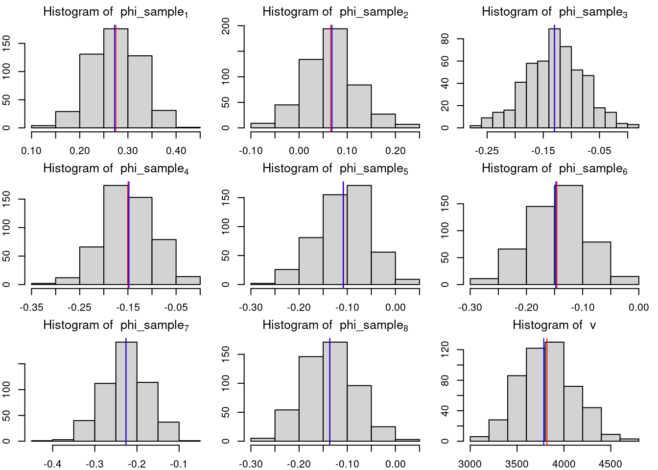
phi should be:
0.2732092 -0.1584926 -0.1398177 -0.1362393
-0.1432613 -0.2306927 -0.194208 -0.2684075
v should be:
3776
```{r}
#| label: lbl-eeg-plot-ar8
## plot histogram of posterior samples of phi and nu
par(mfrow = c(3, 3),
 mar = c(2, 2, 2, 1),  # tight margins
 cex.lab = 1.3)


for(i in 1:p){
  hist(phi_sample[, i], xlab = bquote(phi),
       main = bquote("Histogram of "~phi_sample[.(i)]))
  abline(v = phi_hat[i], col = 'red')
  abline(v = phi_MLE[i], col = 'blue')
}

hist(v_sample, xlab = bquote(nu), main = bquote("Histogram of "~v))
abline(v = v_hat, col = 'red')
abline(v = s2, col = 'blue')
```
```{r}
#| label: lbl-eeg-reciprocal-roots
#phi=phi_MLE
phi=phi_hat
roots=1/polyroot(c(1, -phi)) # compute reciprocal characteristic roots
r=Mod(roots)
# compute moduli of reciprocal roots
lambda=2*pi/Arg(roots) # compute periods of reciprocal roots
# print results modulus and frequency by decreasing order
print(cbind(r, abs(lambda))[order(r, decreasing=TRUE), ][c(2,4,6,8),])
```
the moduli should be:
[1,] 0.9780549
[2,] 0.8658228
[3,] 0.7840114
[4,] 0.7803378
the periods should be:
[1,] 12.124565
[2,] 5.121583
[3,] 2.305216
[4,] 3.224417