## create list for matrices
set_up_dlm_matrices_unknown_v <- function(Ft, Gt, Wt_star){
  if(!is.array(Gt)){
    Stop("Gt and Ft should be array")
  }
  if(missing(Wt_star)){
    return(list(Ft=Ft, Gt=Gt))
  }else{
    return(list(Ft=Ft, Gt=Gt, Wt_star=Wt_star))
  }
}


## create list for initial states
set_up_initial_states_unknown_v <- function(m0, C0_star, n0, S0){
  return(list(m0=m0, C0_star=C0_star, n0=n0, S0=S0))
}

forward_filter_unknown_v <- function(data, matrices,
                              initial_states, delta){
  ## retrieve dataset
  yt <- data$yt
  T<- length(yt)

  ## retrieve matrices
  Ft <- matrices$Ft
  Gt <- matrices$Gt
  if(missing(delta)){
    Wt_star <- matrices$Wt_star
  }

  ## retrieve initial state
  m0 <- initial_states$m0
  C0_star <- initial_states$C0_star
  n0 <- initial_states$n0
  S0 <- initial_states$S0
  C0 <- S0*C0_star

  ## create placeholder for results
  d <- dim(Gt)[1]
  at <- matrix(0, nrow=T, ncol=d)
  Rt <- array(0, dim=c(d, d, T))
  ft <- numeric(T)
  Qt <- numeric(T)
  mt <- matrix(0, nrow=T, ncol=d)
  Ct <- array(0, dim=c(d, d, T))
  et <- numeric(T)
  nt <- numeric(T)
  St <- numeric(T)
  dt <- numeric(T)

  # moments of priors at t
  for(i in 1:T){
    if(i == 1){
      at[i, ] <- Gt[, , i] %*% m0
      Pt <- Gt[, , i] %*% C0 %*% t(Gt[, , i])
      Pt <- 0.5*Pt + 0.5*t(Pt)
      if(missing(delta)){
        Wt <- Wt_star[, , i]*S0
        Rt[, , i] <- Pt + Wt
        Rt[,,i] <- 0.5*Rt[,,i]+0.5*t(Rt[,,i])
      }else{
        Rt[, , i] <- Pt/delta
        Rt[,,i] <- 0.5*Rt[,,i]+0.5*t(Rt[,,i])
      }

    }else{
      at[i, ] <- Gt[, , i] %*% t(mt[i-1, , drop=FALSE])
      Pt <- Gt[, , i] %*% Ct[, , i-1] %*% t(Gt[, , i])
      if(missing(delta)){
        Wt <- Wt_star[, , i] * St[i-1]
        Rt[, , i] <- Pt + Wt
        Rt[,,i]=0.5*Rt[,,i]+0.5*t(Rt[,,i])
      }else{
        Rt[, , i] <- Pt/delta
        Rt[,,i] <- 0.5*Rt[,,i]+0.5*t(Rt[,,i])
      }
    }

    # moments of one-step forecast:
    ft[i] <- t(Ft[, , i]) %*% t(at[i, , drop=FALSE])
    Qt[i] <- t(Ft[, , i]) %*% Rt[, , i] %*% Ft[, , i] +
      ifelse(i==1, S0, St[i-1])
    et[i] <- yt[i] - ft[i]

    nt[i] <- ifelse(i==1, n0, nt[i-1]) + 1
    St[i] <- ifelse(i==1, S0,
                    St[i-1])*(1 + 1/nt[i]*(et[i]^2/Qt[i]-1))

    # moments of posterior at t:
    At <- Rt[, , i] %*% Ft[, , i] / Qt[i]

    mt[i, ] <- at[i, ] + t(At) * et[i]
    Ct[, , i] <- St[i]/ifelse(i==1, S0,
                  St[i-1])*(Rt[, , i] - Qt[i] * At %*% t(At))
    Ct[,,i] <- 0.5*Ct[,,i]+0.5*t(Ct[,,i])
  }
  cat("Forward filtering is completed!\n")
  return(list(mt = mt, Ct = Ct,  at = at, Rt = Rt,
              ft = ft, Qt = Qt,  et = et,
              nt = nt, St = St))
}

### smoothing function ###
backward_smoothing_unknown_v <- function(data, matrices,
                                posterior_states,delta){
  ## retrieve data
  yt <- data$yt
  T <- length(yt)

  ## retrieve matrices
  Ft <- matrices$Ft
  Gt <- matrices$Gt

  ## retrieve matrices
  mt <- posterior_states$mt
  Ct <- posterior_states$Ct
  Rt <- posterior_states$Rt
  nt <- posterior_states$nt
  St <- posterior_states$St
  at <- posterior_states$at

  ## create placeholder for posterior moments
  mnt <- matrix(NA, nrow = dim(mt)[1], ncol = dim(mt)[2])
  Cnt <- array(NA, dim = dim(Ct))
  fnt <- numeric(T)
  Qnt <- numeric(T)

  for(i in T:1){
    if(i == T){
      mnt[i, ] <- mt[i, ]
      Cnt[, , i] <- Ct[, , i]
    }else{
      if(missing(delta)){
        inv_Rtp1 <- chol2inv(chol(Rt[, , i+1]))
        Bt <- Ct[, , i] %*% t(Gt[, , i+1]) %*% inv_Rtp1
        mnt[i, ] <- mt[i, ] + Bt %*% (mnt[i+1, ] - at[i+1, ])
        Cnt[, , i] <- Ct[, , i] + Bt %*% (Cnt[, , i+1] -
                                    Rt[, , i+1]) %*% t(Bt)
        Cnt[,,i] <- 0.5*Cnt[,,i]+0.5*t(Cnt[,,i])
      }else{
        inv_Gt <- solve(Gt[, , i+1])
        mnt[i, ] <- (1-delta)*mt[i, ] +
                delta*inv_Gt %*% t(mnt[i+1, ,drop=FALSE])
        Cnt[, , i] <- (1-delta)*Ct[, , i] +
                delta^2*inv_Gt %*% Cnt[, , i + 1]  %*% t(inv_Gt)
        Cnt[,,i] <- 0.5*Cnt[,,i]+0.5*t(Cnt[,,i])
      }
    }
    fnt[i] <- t(Ft[, , i]) %*% t(mnt[i, , drop=FALSE])
    Qnt[i] <- t(Ft[, , i]) %*% t(Cnt[, , i]) %*% Ft[, , i]
  }
  for(i in 1:T){
     Cnt[,,i]=St[T]*Cnt[,,i]/St[i]
     Qnt[i]=St[T]*Qnt[i]/St[i]
  }
  cat("Backward smoothing is completed!\n")
  return(list(mnt = mnt, Cnt = Cnt, fnt=fnt, Qnt=Qnt))
}

## Forecast Distribution for k step
forecast_function_unknown_v <- function(posterior_states, k,
                                        matrices, delta){

  ## retrieve matrices
  Ft <- matrices$Ft
  Gt <- matrices$Gt
  if(missing(delta)){
    Wt_star <- matrices$Wt_star
  }

  mt <- posterior_states$mt
  Ct <- posterior_states$Ct
  St <- posterior_states$St
  at <- posterior_states$at

  ## set up matrices
  T <- dim(mt)[1] # time points
  d <- dim(mt)[2] # dimension of state parameter vector

  ## placeholder for results
  at <- matrix(NA, nrow = k, ncol = d)
  Rt <- array(NA, dim=c(d, d, k))
  ft <- numeric(k)
  Qt <- numeric(k)

  for(i in 1:k){
    ## moments of state distribution
    if(i == 1){
      at[i, ] <- Gt[, , T+i] %*% t(mt[T, , drop=FALSE])

      if(missing(delta)){
       Rt[, , i] <- Gt[, , T+i] %*% Ct[, , T] %*%
         t(Gt[, , T+i]) + St[T]*Wt_star[, , T+i]
      }else{
        Rt[, , i] <- Gt[, , T+i] %*% Ct[, , T] %*%
          t(Gt[, , T+i])/delta
      }
      Rt[,,i] <- 0.5*Rt[,,i]+0.5*t(Rt[,,i])

    }else{
      at[i, ] <- Gt[, , T+i] %*% t(at[i-1, , drop=FALSE])
      if(missing(delta)){
        Rt[, , i] <- Gt[, , T+i] %*% Rt[, , i-1] %*%
          t(Gt[, , T+i]) + St[T]*Wt_star[, , T + i]
      }else{
        Rt[, , i] <- Gt[, , T+i] %*% Rt[, , i-1] %*%
          t(Gt[, , T+i])/delta
      }
      Rt[,,i] <- 0.5*Rt[,,i]+0.5*t(Rt[,,i])
    }


    ## moments of forecast distribution
    ft[i] <- t(Ft[, , T+i]) %*% t(at[i, , drop=FALSE])
    Qt[i] <- t(Ft[, , T+i]) %*% Rt[, , i] %*% Ft[, , T+i] +
      St[T]
  }
  cat("Forecasting is completed!\n") # indicator of completion
  return(list(at=at, Rt=Rt, ft=ft, Qt=Qt))
}

## obtain 95% credible interval
get_credible_interval_unknown_v <- function(ft, Qt, nt,
                                   quantile = c(0.025, 0.975)){
  bound <- matrix(0, nrow=length(ft), ncol=2)

  if ((length(nt)==1)){
   for (t in 1:length(ft)){
      t_quantile <- qt(quantile[1], df = nt)
      bound[t, 1] <- ft[t] + t_quantile*sqrt(as.numeric(Qt[t]))

  # upper bound of 95% credible interval
      t_quantile <- qt(quantile[2], df = nt)
      bound[t, 2] <- ft[t] +
        t_quantile*sqrt(as.numeric(Qt[t]))}
  }else{
  # lower bound of 95% credible interval
    for (t in 1:length(ft)){
      t_quantile <- qt(quantile[1], df = nt[t])
      bound[t, 1] <- ft[t] +
        t_quantile*sqrt(as.numeric(Qt[t]))

  # upper bound of 95% credible interval
      t_quantile <- qt(quantile[2], df = nt[t])
      bound[t, 2] <- ft[t] +
        t_quantile*sqrt(as.numeric(Qt[t]))}
  }
  return(bound)

}
Noteopen issues
Is there a recommended way to recover the parameter vector from the model object?
the question about this dimension of Theta seems to be as follows for seasonal component p = 2m-1 so we get 2(3)-1=5. The problem is that it isn’t clear that p here is the number of frequencies/harmonics. The linear trend component has 1 parameter
101.1 Practice Graded Assignment: NDLM data analysis
This peer-reviewed activity is highly recommended. It does not figure into your grade for this course, but it does provide you with the opportunity to apply what you’ve learned in R and prepare you for your data analysis project in week 5.
The R code below fits a Normal Dynamic Linear Model to the monthly time series of Google trends “hits” for the term “time series”. The model has two components:
- a polynomial model of order 2 and
- a seasonal component with 4 frequencies:
- \omega_1=2\pi/12, (annual cycle)
- \omega_2=2\pi/6 (6 months cycle),
- \omega_3=2\pi/4 and
- \omega_4=2\pi/3.
The model assumes that the observational variance v is unknown and the system variance-covariance matrix W_t is specified using a single discount factor. The discount factor is chosen using an optimality criterion as explained in the course.
You will be asked to modify the code in order to consider a DLM with two components:
- a polynomial model of order 1 and
- a seasonal component that contains a fundamental period of p = 12 and 2 additional harmonics for a total of 3 frequencies: \omega1=2\pi/12, \omega2=2\pi/6 and \omega3=2\pi/4.
You will also need to optimize the choice of the discount factor for this model.
You will be asked to upload pictures summarizing your results.
R code to fit the model:
- requires R packages
gtrends,anddlmas well as the files- “all_dlm_functions_unknown_v.R” and
- “discountfactor_selection_functions.R” also provided below.
101.1.1 All dlm functions unknown v
101.1.2 Discount factor selection functions
##################################################
##### using discount factor ##########
##################################################
## compute measures of forecasting accuracy
## MAD: mean absolute deviation
## MSE: mean square error
## MAPE: mean absolute percentage error
## Neg LL: Negative log-likelihood of disc,
##         based on the one step ahead forecast distribution
measure_forecast_accuracy <- function(et, yt, Qt=NA, nt=NA, type){
  if(type == "MAD"){
    measure <- mean(abs(et))
  }else if(type == "MSE"){
    measure <- mean(et^2)
  }else if(type == "MAPE"){
    measure <- mean(abs(et)/yt)
  }else if(type == "NLL"){
    measure <- log_likelihood_one_step_ahead(et, Qt, nt)
  }else{
    stop("Wrong type!")
  }
  return(measure)
}


## compute log likelihood of one step ahead forecast function
log_likelihood_one_step_ahead <- function(et, Qt, nt){
  ## et:the one-step-ahead error
  ## Qt: variance of one-step-ahead forecast function
  ## nt: degrees freedom of t distribution
  T <- length(et)
  aux=0
  for (t in 1:T){
    zt=et[t]/sqrt(Qt[t])
    aux=(dt(zt,df=nt[t],log=TRUE)-log(sqrt(Qt[t]))) + aux
  }
  return(-aux)
}

## Maximize log density of one-step-ahead forecast function to select discount factor
adaptive_dlm <- function(data, matrices, initial_states, df_range, type,
                         forecast=TRUE){
  measure_best <- NA
  measure <- numeric(length(df_range))
  valid_data <- data$valid_data
  df_opt <- NA
  j <- 0
  ## find the optimal discount factor
  for(i in df_range){
    j <- j + 1
    results_tmp <- forward_filter_unknown_v(data, matrices, initial_states, i)

    measure[j] <- measure_forecast_accuracy(et=results_tmp$et, yt=data$yt,
                                  Qt=results_tmp$Qt,
                                  nt=c(initial_states$n0,results_tmp$nt), type=type)


    if(j == 1){
      measure_best <- measure[j]
      results_filtered <- results_tmp
      df_opt <- i
    }else if(measure[j] < measure_best){
      measure_best <- measure[j]
      results_filtered <- results_tmp
      df_opt <- i
    }
  }
  results_smoothed <- backward_smoothing_unknown_v(data, matrices, results_filtered, delta = df_opt)
  if(forecast){
    results_forecast <- forecast_function(results_filtered, length(valid_data),
                                          matrices, df_opt)
    return(list(results_filtered=results_filtered,
                results_smoothed=results_smoothed,
                results_forecast=results_forecast,
                df_opt = df_opt, measure=measure))
  }else{
    return(list(results_filtered=results_filtered,
                results_smoothed=results_smoothed,
                df_opt = df_opt, measure=measure))
  }

}
101.1.3 Grading Criteria
The assignment will be graded based on the uploaded pictures summarizing the results. Estimates of some of the model parameters and additional discussion will also be requested.
# --- Clean helper ---
clean_gtrends <- function(df, lt1_value = 0.5) {
  # Map "<1" to a numeric (choose 0, 0.5, or 1; 0.5 is a common midpoint choice)
  df$hits <- as.numeric(ifelse(df$hits == "<1", lt1_value, df$hits))
  # Ensure date is Date (works fine in base plot)
  df$date <- as.Date(df$date)
  # Drop rows with missing/invalid values
  df <- df[is.finite(df$hits) & !is.na(df$date), ]
  rownames(df) <- NULL
  df
}
#| label: code-gtrendsR-get-data
# download data
library(gtrendsR)
timeseries_data<-gtrends("time series",time="all",hl="en",geo="",onlyInterest=TRUE)
#timeseries_data <- gtrends(c("NHL", "NFL"), time = "today 1-m")
#timeseries_data <- gtrends(keyword = "obama",geo = "US-AL-630",time = "today 1-m")
plot(timeseries_data$interest_over_time)
names(timeseries_data)
timeseries_data=timeseries_data$interest_over_time
data=list(yt=timeseries_data$hits)
plot(data$yt, type='l', main="Google Trends: time series",
xlab='time', ylab='Google hits', lty=3, ylim=c(0,100))
ts <- clean_gtrends(ts, lt1_value = 0.5)
write.csv(ts, "google_trends_timeseries.csv", row.names = FALSE)loaded_csv <- read.csv("google_trends_timeseries.csv",stringsAsFactors = FALSE)
loaded_csv <- clean_gtrends(loaded_csv, lt1_value = 0.5)
data=list(yt=loaded_csv$hits,date=loaded_csv$date)
plot(loaded_csv$date, loaded_csv$hits, type = 'l', main = "Google Trends: time series (Loaded)",
xlab = 'Time', ylab = 'Google hits', lty = 3, ylim = c(0,100))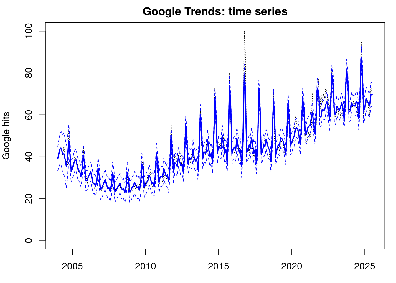
library(dlm)
model_seasonal=dlmModTrig(s=12,q=4,dV=0,dW=1)
model_trend=dlmModPoly(order=2,dV=10,dW=rep(1,2),m0=c(40,0))
model=model_trend+model_seasonal
model$C0=10*diag(10)
n0=1
S0=10
k=length(model$m0)
T=length(data$yt)

Ft=array(0,c(1,k,T))
Gt=array(0,c(k,k,T))
for(t in 1:T){
   Ft[,,t]=model$FF
   Gt[,,t]=model$GG
}

source('all_dlm_functions_unknown_v.R')
source('discountfactor_selection_functions.R')

matrices=set_up_dlm_matrices_unknown_v(Ft=Ft,Gt=Gt)
initial_states=set_up_initial_states_unknown_v(model$m0,
                                               model$C0,n0,S0)

df_range=seq(0.9,1,by=0.005)

## fit discount DLM
## MSE
results_MSE <- adaptive_dlm(data, matrices,
               initial_states, df_range,"MSE",forecast=FALSE)
Forward filtering is completed!
Forward filtering is completed!
Forward filtering is completed!
Forward filtering is completed!
Forward filtering is completed!
Forward filtering is completed!
Forward filtering is completed!
Forward filtering is completed!
Forward filtering is completed!
Forward filtering is completed!
Forward filtering is completed!
Forward filtering is completed!
Forward filtering is completed!
Forward filtering is completed!
Forward filtering is completed!
Forward filtering is completed!
Forward filtering is completed!
Forward filtering is completed!
Forward filtering is completed!
Forward filtering is completed!
Forward filtering is completed!
Backward smoothing is completed!## print selected discount factor
print(paste("The selected discount factor:",results_MSE$df_opt))[1] "The selected discount factor: 0.955"## retrieve filtered results
results_filtered <- results_MSE$results_filtered
ci_filtered <- get_credible_interval_unknown_v(
results_filtered$ft,results_filtered$Qt,results_filtered$nt)
## retrieve smoothed results
results_smoothed <- results_MSE$results_smoothed
ci_smoothed <- get_credible_interval_unknown_v(
results_smoothed$fnt, results_smoothed$Qnt,
results_filtered$nt[length(results_smoothed$fnt)])
## plot smoothing results
par(mfrow=c(1,1), mar = c(3, 4, 2, 1))
index <- data$date
plot(index, data$yt, ylab='Google hits',
main = "Google Trends: time series", type = 'l',
xlab = 'time', lty=3,ylim=c(0,100))
lines(index, results_smoothed$fnt, type = 'l', col='blue',
lwd=2)
lines(index, ci_smoothed[, 1], type='l', col='blue', lty=2)
lines(index, ci_smoothed[, 2], type='l', col='blue', lty=2)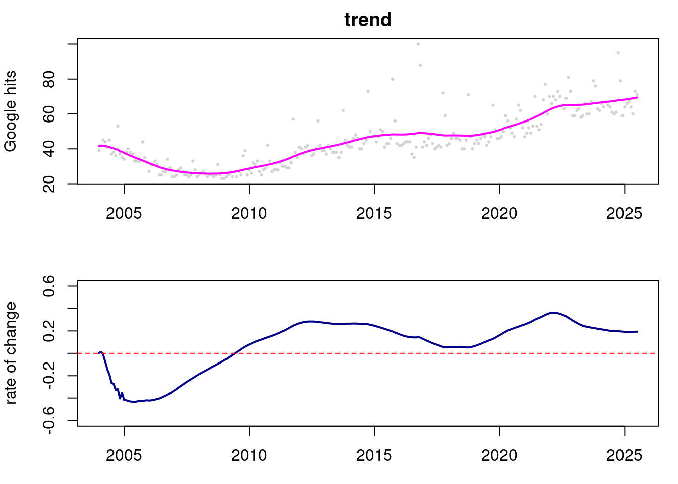
# Plot trend and rate of change
par(mfrow=c(2,1), mar = c(3, 4, 2, 1))
plot(index,data$yt,pch=19,cex=0.3,col='lightgray',xlab="time",
     ylab="Google hits",main="trend")
lines(index,results_smoothed$mnt[,1],lwd=2,col='magenta')
plot(index,results_smoothed$mnt[,2],col='darkblue',lwd=2,
     type='l', ylim=c(-0.6,0.6), xlab="time",
     ylab="rate of change")
abline(h=0,col='red',lty=2)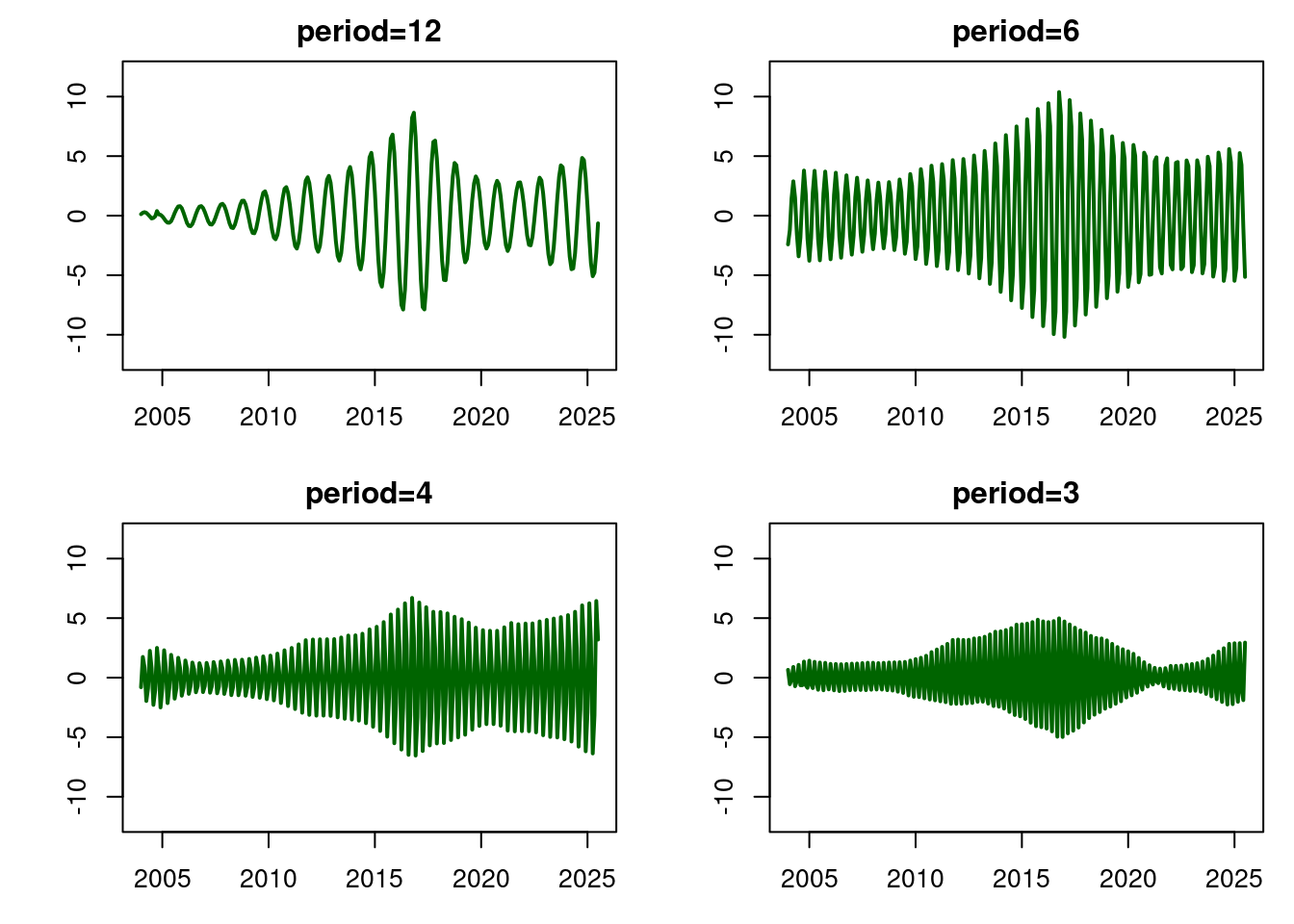
# Plot seasonal components
par(mfrow=c(2,2), mar = c(3, 4, 2, 1))
plot(index,results_smoothed$mnt[,3],lwd=2,col="darkgreen",
     type='l', xlab="time",ylab="",main="period=12",
     ylim=c(-12,12))
plot(index,results_smoothed$mnt[,5],lwd=2,col="darkgreen",
     type='l',xlab="time",ylab="",main="period=6",
     ylim=c(-12,12))
plot(index,results_smoothed$mnt[,7],lwd=2,col="darkgreen",
     type='l', xlab="time",ylab="",main="period=4",
     ylim=c(-12,12))
plot(index,results_smoothed$mnt[,9],lwd=2,col="darkgreen",
     type='l', xlab="time",ylab="",main="period=3",
     ylim=c(-12,12))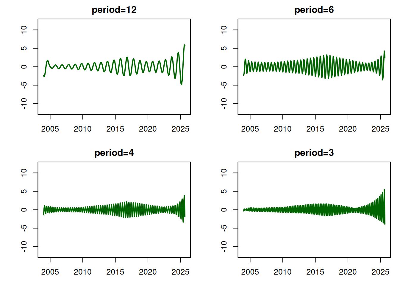
#Estimate for the observational variance: St[T]
results_filtered$St[T]
[1] 17.89918101.2 My Submission
What modifications to the lines of R-code below have to be made to consider a DLM with the following structure:
- a polynomial model of order 1 and
- a seasonal component that contains a fundamental period of p=12 and 2 additional harmonics for a total of 3 frequencies: \omega_1=2\pi/12, \omega_2=2\pi/6 and \omega_3=2\pi/4.?
Upload the revised lines of R code (in rich text format, not as an R file), that provide the structure of the new model.
Assume dV=0, dW=1 in the seasonal component, dV=10,dW=1,m_0=40,C_0=10I,n_0=1,S0=10 with I being identity matrix with the appropriate dimensions n0=1 and S0=10
library(dlm)
model_seasonal=dlmModTrig(s=12,q=4,dV=0,dW=1)
model_trend=dlmModPoly(order=2,dV=10,dW=rep(1,2),m0=c(40,0))
model=model_trend+model_seasonal
model$C0=10*diag(10)
n0=1
S0=10
answer:
library(dlm)
model_seasonal=dlmModTrig(s=12,q=3,dV=0,dW=1)
model_trend=dlmModPoly(order=1,dV=10,dW=rep(1,1),m0=c(40))
model=model_trend+model_seasonal # superposition
model$C0=10*diag(7)
n0=1
S0=10
The new DLM with has the following structure: (a) a polynomial model of order 1 and (b) a seasonal component that contains a fundamental period of p=12 and 2 additional harmonics for a total of 3 frequencies: \omega_1=2\pi/12, \omega_2=2\pi/6 and \omega_3=2\pi/4.
What is the dimension of the state parameter vector _t for this new model that accounts for both components (a) and (b)?
# Dimension of the state parameter vector _t
cat(model$C10) # 3 freqs * 2 states from seasonal + 1 from trendk=length(model$m0)
T=length(data$yt)
Ft=array(0,c(1,k,T))
Gt=array(0,c(k,k,T))
for(t in 1:T){
Ft[,,t]=model$FF
Gt[,,t]=model$GG
}
source('all_dlm_functions_unknown_v.R')
source('discountfactor_selection_functions.R')
matrices=set_up_dlm_matrices_unknown_v(Ft=Ft,Gt=Gt)
initial_states=set_up_initial_states_unknown_v(model$m0,
model$C0,n0,S0)
df_range=seq(0.9,1,by=0.005)
## fit discount DLM
## MSE
results_MSE <- adaptive_dlm(data, matrices,
initial_states, df_range,"MSE",forecast=FALSE)Forward filtering is completed!
Forward filtering is completed!
Forward filtering is completed!
Forward filtering is completed!
Forward filtering is completed!
Forward filtering is completed!
Forward filtering is completed!
Forward filtering is completed!
Forward filtering is completed!
Forward filtering is completed!
Forward filtering is completed!
Forward filtering is completed!
Forward filtering is completed!
Forward filtering is completed!
Forward filtering is completed!
Forward filtering is completed!
Forward filtering is completed!
Forward filtering is completed!
Forward filtering is completed!
Forward filtering is completed!
Forward filtering is completed!
Backward smoothing is completed!## print selected discount factor
print(paste("The selected discount factor:",results_MSE$df_opt))[1] "The selected discount factor: 0.92"## retrieve filtered results
results_filtered <- results_MSE$results_filtered
ci_filtered <- get_credible_interval_unknown_v(
results_filtered$ft,results_filtered$Qt,results_filtered$nt)
## retrieve smoothed results
results_smoothed <- results_MSE$results_smoothed
ci_smoothed <- get_credible_interval_unknown_v(
results_smoothed$fnt, results_smoothed$Qnt,
results_filtered$nt[length(results_smoothed$fnt)])## plot smoothing results
par(mfrow=c(1,1), mar = c(3, 4, 2, 1))
index <- data$date
plot(index, data$yt, ylab='Google hits',
main = "Google Trends: time series", type = 'l',
xlab = 'time', lty=3,ylim=c(0,100))
lines(index, results_smoothed$fnt, type = 'l', col='blue', lwd=2)
lines(index, ci_smoothed[, 1], type='l', col='blue', lty=2)
lines(index, ci_smoothed[, 2], type='l', col='blue', lty=2)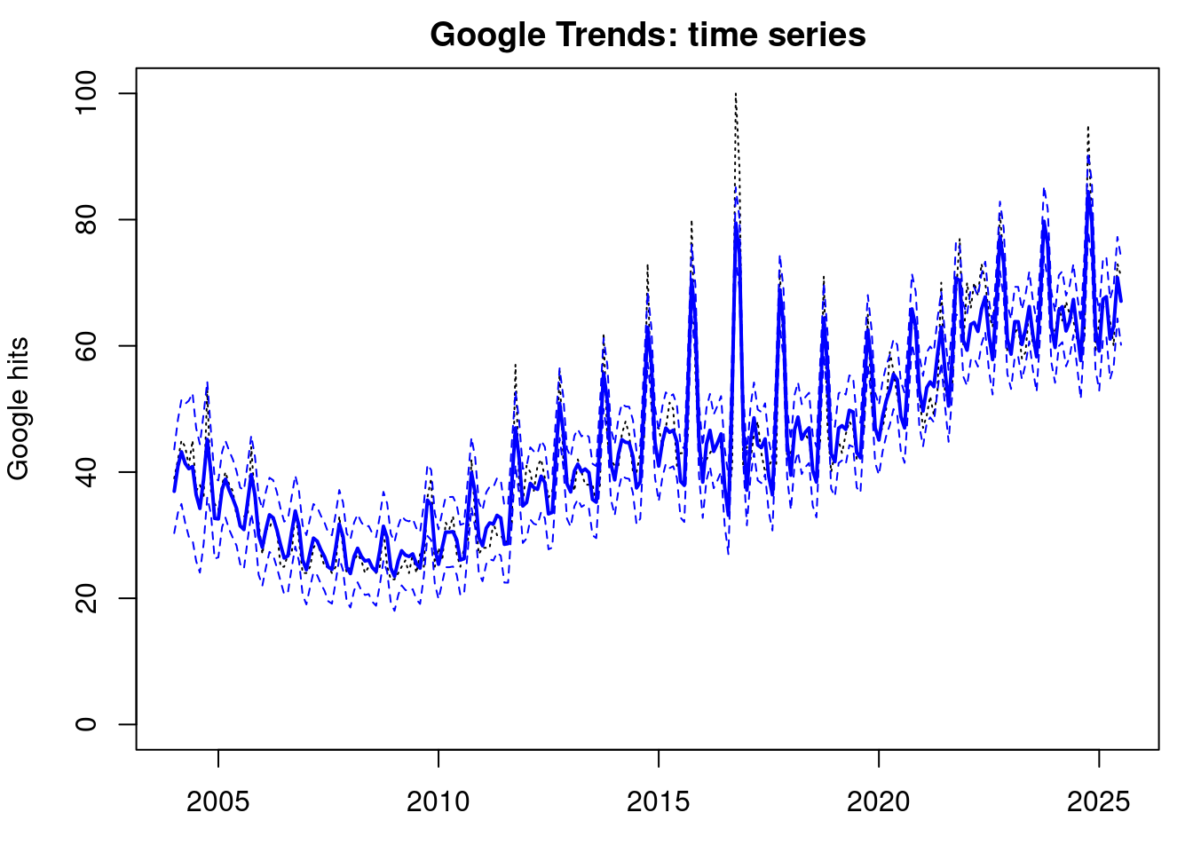
# Plot trend and rate of change
par(mfrow=c(2,1), mar = c(3, 4, 2, 1))
plot(index,data$yt,pch=19,cex=0.3,col='lightgray',xlab="time",
     ylab="Google hits",main="trend")
lines(index,results_smoothed$mnt[,1],lwd=2,col='magenta')
plot(index,results_smoothed$mnt[,2],col='darkblue',lwd=2,
     type='l', ylim=c(-0.6,0.6), xlab="time",
     ylab="rate of change")
abline(h=0,col='red',lty=2)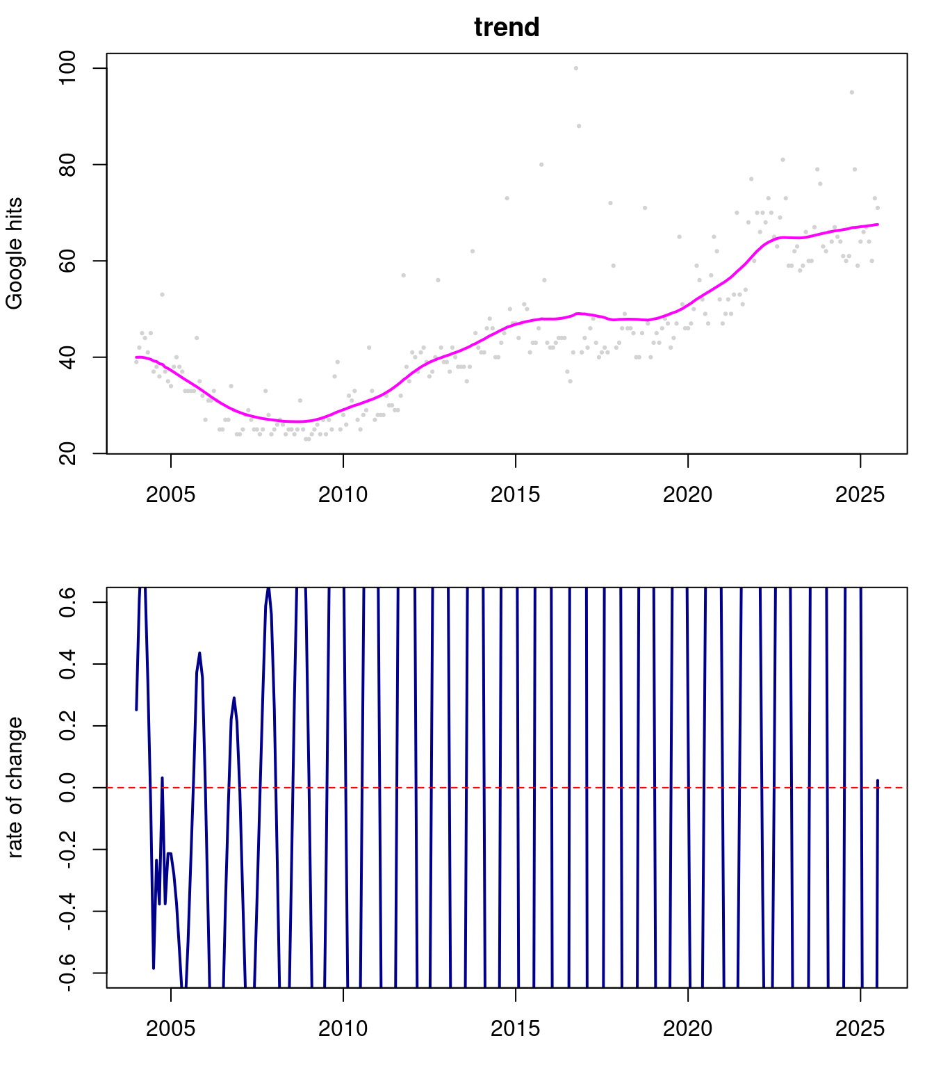
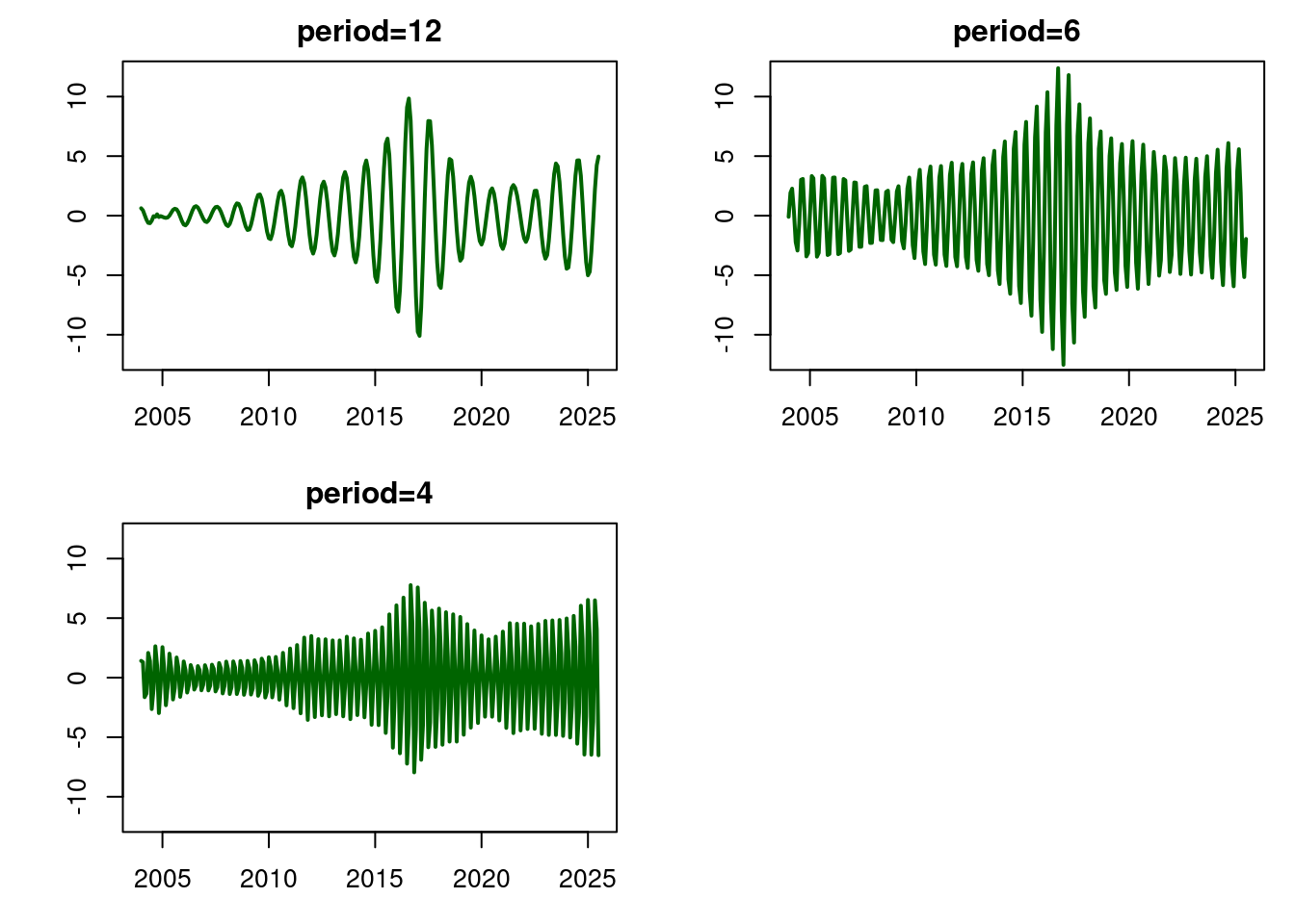
# Plot seasonal components
par(mfrow=c(2,2), mar = c(3, 4, 2, 1))
plot(index,results_smoothed$mnt[,3],lwd=2,col="darkgreen",
     type='l', xlab="time",ylab="",main="period=12",
     ylim=c(-12,12))
plot(index,results_smoothed$mnt[,5],lwd=2,col="darkgreen",
     type='l',xlab="time",ylab="",main="period=6",
     ylim=c(-12,12))
plot(index,results_smoothed$mnt[,7],lwd=2,col="darkgreen",
     type='l', xlab="time",ylab="",main="period=4",
     ylim=c(-12,12))
# plot(index,results_smoothed$mnt[,9],lwd=2,col="darkgreen",
#      type='l', xlab="time",ylab="",main="period=3",
#      ylim=c(-12,12))

#Estimate for the observational variance: St[T]
results_filtered$St[T]
[1] 17.55156