set.seed(123)
n <- 100
V <- 1
mu <- 0
y <- mu + rnorm(n, 0, V)
plot(y, type = "l", col = "blue", lwd = 2, xlab = "Time", ylab = "y", main = "Model with no temporal structure")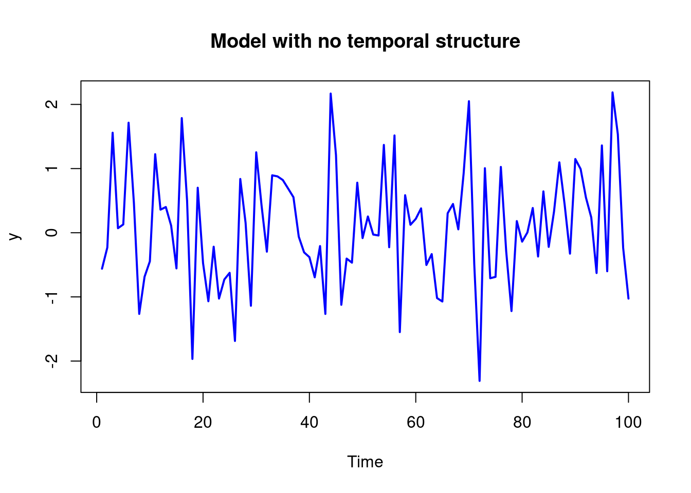
Time Series, Filtering, Kalman filtering, Smoothing, NDLM, Normal Dynamic Linear Models, Polynomial Trend Models, Regression Models, Superposition Principle, R code
Normal Dynamic Linear Models (NDLMs) are defined and illustrated in this module using several examples Model building based on the forecast function via the superposition principle is explained. Methods for Bayesian filtering, smoothing and forecasting for NDLMs in the case of known observational variances and known system covariance matrices are discussed and illustrated..
The Normal Dynamic Linear Model (DLM) is covered (R. Prado, Ferreira, and West 2023, 117–44)
In this module, we will motivate and develop a class of models suitable for for analyzing and forecasting non-stationary time series called normal dynamic linear models . We will talk about Bayesian inference and forecasting within this class of models and describe model building as well.
Let’s begin with a very simple model that has no temporal structure, just a mean value with some variation that is:
y_t = \mu + v_t \qquad v_t \overset{\text{iid}}{\sim} \mathcal{N}(0, \nu) \qquad \text{(white noise model)} \tag{97.1}
where:
If we plot this model we might see the following graph:
set.seed(123)
n <- 100
V <- 1
mu <- 0
y <- mu + rnorm(n, 0, V)
plot(y, type = "l", col = "blue", lwd = 2, xlab = "Time", ylab = "y", main = "Model with no temporal structure")For this model the mean of the time series is \mu will be the the expected value of y_t, which is \mu. And the variance of y_t is \nu.
\mathbb{E}[y_t] = \mu \qquad \text{and} \qquad \mathbb{V}ar[y_t] = \nu \qquad \tag{97.2}
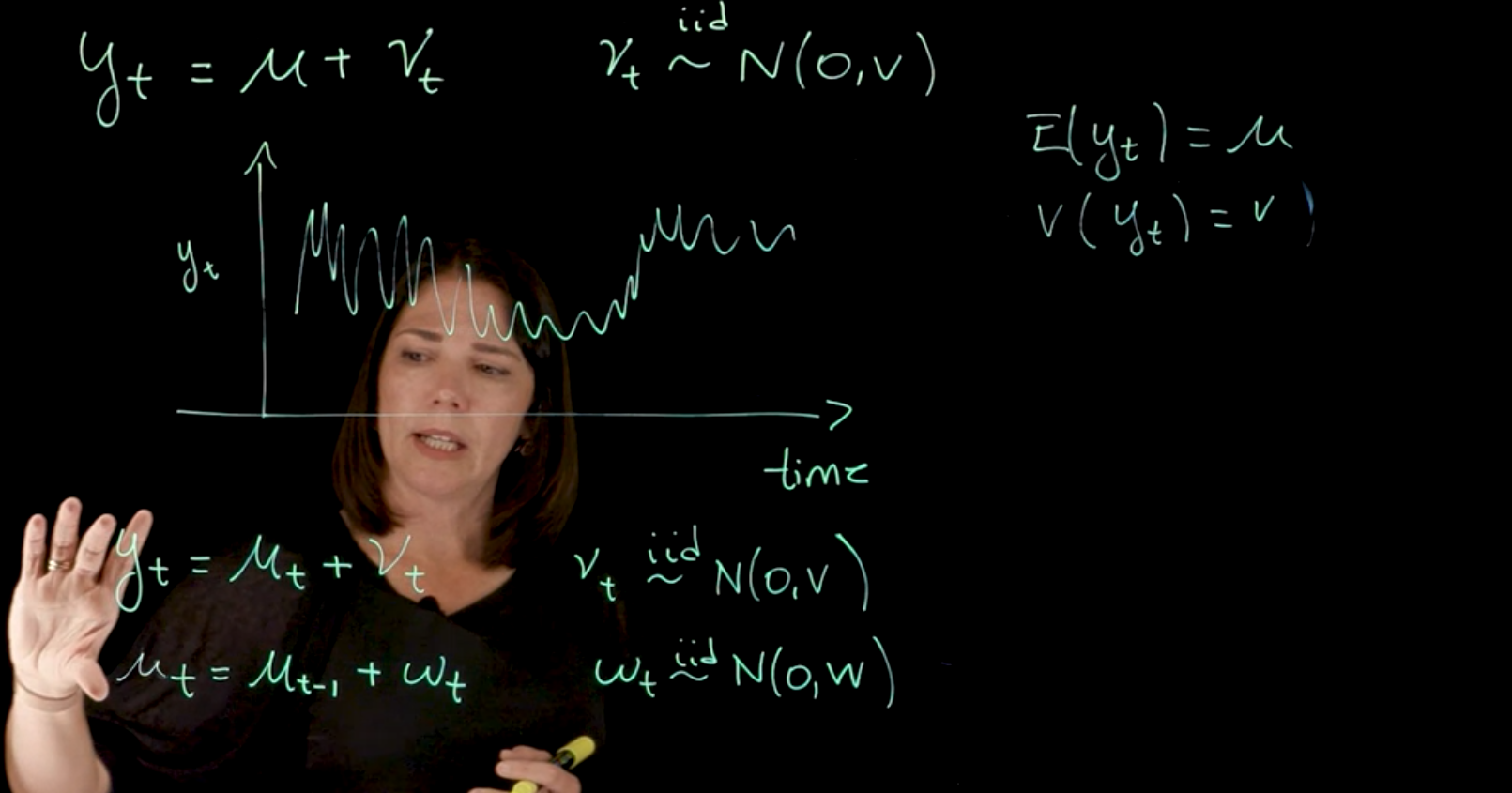
Next we incorporate some temporal structure, we allow the expected value of the time series, to change over time. To can achieve this, by update the model definition with a \mu_t where the index indicates that it can change at every time step. And let us keep the noise unchanged. i.e. we set it to \mu_t \in N(0,\nu).
We get the following model:
y_t = \mu_t + \nu_t \quad \nu_t \overset{\text{iid}}{\sim} N(0, V) \qquad \text{(radom walk model)} \tag{97.3}
To complete this we need to also decide how to incorporate the the changes over time in the parameter \mu_t. We might consider different options but we should pick the simplest possible to start with. One option is to assume that the expected value of \mu_t is just the expected value of \mu_{t-1} plus some noise.
We now have that random walk type of structure where \mu_t can be written in terms of \mu(t-1). The expected value of \mu_t, we can think of it as \mu_{t-1} + \text{some noise}. This error is once again, assumed to be normally distributed random variable centered at zero and with variance W. Another assumption that we have made here is that the \nu_t and \omega_t, are also independent of each other.
putting this together we get:
\begin{aligned} y_t &= \mu_t + \nu_t & \nu_t & \overset{\text{iid}}{\sim} \mathcal{N}(0, V) & \text{(Observation eq.)} \\ \mu_t &= \mu_{t-1} + \omega_t & \omega_t & \overset{\text{iid}}{\sim} \mathcal{N}(0, W) & \text{(System/evolution eq.)} \end{aligned} \tag{97.4}
With this model, what we are assuming is that the mean level of the series is changing over time. Note that this is an example of a Gaussian or Normal dynamic linear model.
NDLMs are a two level hierarchical models where :
This is our first example. Next we will be discuss the general class of models. Later we will consider how to incorporate different structures into the model, and how to perform Bayesian inference for filtering smoothing and forecasting.
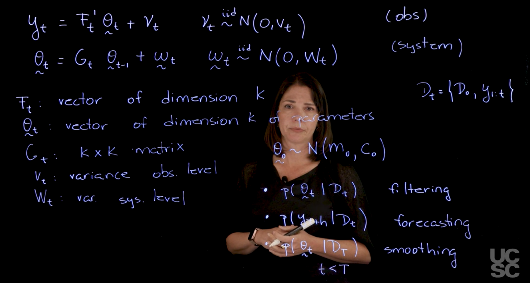
The general class of dynamic linear models can be written as follows:
We are going to have two equations. One is the so-called observation equation that relates the observations to the parameters in the model, and the notation we are going to use is as follows.
\begin{aligned} y_t &= \vec{F}_t' \vec{\theta}_t + \nu_t && \nu_t \overset{\text{iid}}{\sim} \mathcal{N}(0, V_t) && \text{(obs)} \\ \vec{\theta}_t &= G_t \vec{\theta}_{t-1} + \vec{\omega}_t && \vec{\omega}_t \overset{\text{iid}}{\sim} \mathcal{N}(0, W_t) && \text{(system)} \end{aligned} \tag{97.5}
Where:
We also have the prior distribution for the state vector at time 0:
In terms of the inference, there are a few different kinds of densities and quantities that we are interested in:
One of the distributions that we are interested in finding is the so-called filtering distribution. We may be interested here in finding what is the density of \theta_t given all the observations that we have up to time t.
\mathcal{D}_t= \{\mathcal{D}_0, y_{1:T}\} \tag{97.6}
We will denote information as \mathcal{D}_t. Usually, it is all the information we have at time zero (i.e. our prior), coupled with all the data points I have up to time t.
Here we conditioning on all the observed quantities and the prior information up to time t, and I may be interested in just finding what is the distribution for \theta_t. This is called filtering.
\mathbb{P}r(\theta_t \mid \mathcal{D}_t) \qquad \text{filtering distribution} \tag{97.7}
Another distribution that is very important in time series analysis is the forecasting distribution. We may be interested in the distribution of y{t+h}? where we consider h lags into the future and we have all the information \mathcal{D}_t, up to time t. We want to do a predictions here
\mathbb{P}r(y_{t+h} \mid \mathcal{D}_t) \qquad \text{forecasting distribution} \tag{97.8}
Another important quantity or an important set of distributions is what we call the smoothing distribution. Usually, you have a time series, when you get your data, you observe, I don’t know, 300 data points. As you go with the filtering, you are going to start from zero all the way to 300 and you’re going to update these filtering distributions as you go and move forward. We may want instead to revisit the parameter at time 10, for example, given that you now have observed all these 300 observations. In that case, you’re interested in densities that are of the form. Let’s say that you observe capital T in your process and now you are going to revisit that density for \theta_t. This is now in the past. Here we assume that t<T. This is called smoothing.
So you have more observation once you have seen the data. We will talk about how to perform Bayesian inference to obtain all these distributions under this model setting.
\mathbb{P}r(\theta_t \mid \mathcal{D}_T) \qquad t < T \qquad \text{smoothing distribution} \tag{97.9}
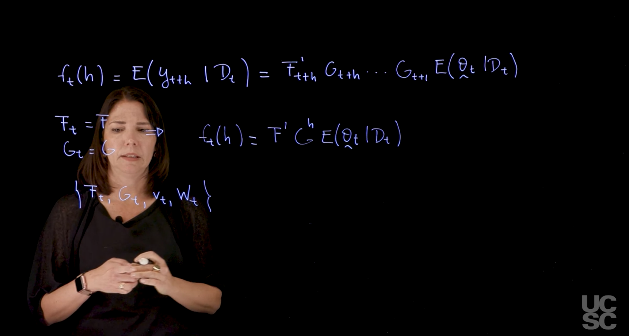
In addition to all the structure that we described before and all the densities that we are interested in finding, we also have as usual, the so-called forecast function, which instead of being the density is just \mathbb{E}[y(t+h)\mid \mathcal{D}_t] i.e. expected value of y at time t given all the information we have before time t.
\mathbb{E}[y(t+h)\mid \mathcal(D_t)] = F'_{t+h} G_{t+h} \ldots G_{t+1} \mathbb{E}[\theta_t \mid \mathcal{D}_t] \tag{97.10}
This is the form of the forecast function.
There are particular cases and particular models that we will be discussing in which the F_t=F, i.e. constant and also G_t = G is also constant for all t. In these cases, the forecast function can be simplified and written as:
f_t(h) = \mathbb{E}(y_{t+h} \mid D_t) = F'G^h \mathbb{E}(\theta_t \mid \mathcal{D}_t) \tag{97.11}
One thing that we will learn is that the eigen-structure of this matrix is very important to define the form of the forecast function, and it’s very important for model building and for adding components into your model.
Finally, just in terms of short notation, we can always write down when we’re working with normal dynamic linear models, we may be referring to the model instead of writing the two equations, the system and the observation equation. I can just write all the components that define my model. \{F_t, G_t, v_t, W_t\} \tag{97.12}
In this part of the course, I will discuss the class of normal dynamic linear models for analyzing and forecasting non-stationary time series. We will talk about Bayesian inference and forecasting within this class of models and describe model building as well.
I want to begin first with a motivating example. Suppose you have a model that is very simple and has no temporal structure here, just a model that looks like this. You have your time series y_t. Then you’re interested in just thinking about what is the mean level of that time series. That mean level, I’m going to call it \mu and then I have some noise and the noise is normally distributed. They are all independent, identically distributed normal random variables \mathcal{N}(0,v). Again, I can think of my time series. Suppose that I have my time series here, and then I’m plotting y_t. Then I have something that looks like this. In this model that \mu is going to try to get the mean of that time series, this expected value of y_t, which is \mu. The variance here of y_t is v under this model. What may happen in practice again, this model has no temporal structure, I may want to incorporate some temporal structure that says, well, I think that the level of this, the expected value of this time series, should be changing over time. If you were to do that, you will write down a model where the \mu changes over time, so it’s indexed in time. Then you have still your same noise here. Let’s again assume \mathcal{N}(0,v). I have now to make a decision on how I’m going to incorporate temporal structure by modeling the changes over time in this parameter \mu_t. You could consider different options.
The simplest possible, probably that you can consider is something that looks like this. You have that random walk type of structure where \mu_t is now going to be written as \mu_{t-1}. The expected value of \mu_t, you’ll think of it as \mu_{t-1} plus some noise. That error here is going to be again, assume normally distributed random variable centered at zero and with variance w. There is another assumption that we can make here and is that the nu t and omega t here, are also independent of each other. When I have this model, what am assuming here is that the mean level of the series is changing over time.
These type of models have a few characteristics. This is an example of a normal dynamic linear model, as we will see later. In this models, we usually have a few things.
The first thing is we have two equations. One is the so-called observation equation that is relating your y_t, your observed process to some parameters in the model that are changing over time. The next equation is the so-called system level equation or evolution equation that tells me how that time varying parameter is going to be changing over time. The other thing you may notice is that we have a linear structure both in the observational level and in the system level. The linear structure, in the sense of the expected value of y_t is just a linear function of that \mu_t. It happens to be \mu_t in this particular case. In the second level, I can think of the expected value of \mu_t as a linear function given \mu_{t-1}, so it’s a function that is linear on \mu_{t-1}. There is that linear structure. The other thing that we have here is at both levels, we have the assumption of normality for the noise terms in those equations. This is an example of a Gaussian or normal dynamic. These are time-varying parameters linear model. We will be discussing the general class of models. This is just an example. We will also discuss how to build different structures into the model, as well as how to perform Bayesian inference and forecasting.
The general class of dynamic linear models can be written as follows. Again, we are going to have two equations. One is the so-called observation equation that relates the observations to the parameters in the model, and the notation we are going to use is as follows. Here, my observations are univariate. We are discussing models for univariate time series. I have that related to a vector of parameters, \theta_t plus some noise here. This is the noise. The noise are assumed to be independent, identically distributed normal random variables, 0, V_t. Then I have another equation which is a system equation that has this form. There is a general G_t matrix. This is going to be depending on \theta_{t-1}. This is a vector, and then I have again, these are iid multivariate \mathcal{N}(0, W_t). This is the observation equation. This is the system equation or evolution equation. This defines a normal dynamic linear model. Here, we are going to say that F_t is a vector. The dimension of the vector is going to be the same as the number of parameters in the model. Let’s say we have k. This is a vector of known values. For each t, we are going to assume that we know what that vector is. Then we have the vector of parameters here is also of dimension k of parameters. The G is the next thing we need to define is a known matrix. That one is also assumed to be known, and then I have V_t is variance at the observational level. The W_t we are going to assume at the beginning that these two quantities are also known for all the values t. This is the variance-covariance matrix at the system level. Again, if we think about these two equations, we have the model defined in this way.
There is a next piece that we need to consider if we are going to perform based in inference for the model parameters. The next piece that we need to consider to just fully specify the model is what is the prior distribution. In a normal dynamic linear model, the prior distribution is assumed to be conjugate here. In the case again in which V_t and W_t are known, we are going to be assuming that, say that zero, the parameter vector before observing any data is going to be normally distributed Multivariate normal with M_0 and C_0. The mean is a vector, again of the same dimension as \theta_0. Then I have k by k covariance matrix there as well. These are assumed to be also given to move forward with the model.
In terms of the inference, there are different kinds of densities and quantities that we are interested in. One distribution that we are interested in finding is the so-called filtering distribution. We may be interested here in finding what is the density of \theta_{t} given all the observations that we have up to time t. I’m going to call and all the information that I have up to time t. I’m going to call that D_t . It can also be, in some cases, I will just write down. So D_t, you can view with all the info up to time t. Usually, it is all the information I have at time zero. Then coupled, if there is no additional information that’s going to be coupled with all the data points I have up to that time. Here I’m conditioning on all the observed quantities and the prior information up to time t, and I may be interested in just finding what is the distribution for \theta_{t}.
This is called filtering. Another quantity that is very important in time series analysis is forecasting.
I may be interested in just what is the density, the distribution of y_{t+h} ? Again, the number of steps ahead here, here I’m thinking of h, given that I have all this information up to time t. I’m interested in predictions here. We will be talking about forecasting. Then another important quantity or an important set of distributions is what we call the smoothing distribution. Usually, you have a time series, when you get your data, you observe, I don’t know, 300 data points. As you go with the filtering, you are going to start from zero all the way to 300 and you’re going to update these filtering distributions as you go and move forward. But then you may want to revisit your parameter at time 10, for example, given that you now have observed all these 300 observations. In that case, you’re interested in densities that are of the form. Let’s say that you observe capital T in your process and now you are going to revisit that density for \theta_t. This is now in the past. Here we assume that t is smaller than capital T. This is called smoothing. So you have more observation once you have seen the data. We will talk about how to perform Bayesian inference to obtain all these distributions under this model setting.
In addition to all the structure that we described before and all the densities that we are interested in finding, we also have as usual, the so-called forecast function, which is just instead of being the density is just expected value of y(t+h) given all the information I have up to time t. In the case of a general normal dynamic linear model, we have the structure for these just using the equations, the observation and the system of equations.
We’re going to have here G_{t+h}. We multiply all these all the way to G_(t+1), and then we have the \mathbb{E}[\theta_{t}\mid D_t]. This is the form of the forecast function. There are particular cases and particular models that we will be discussing in which the F_t is equal to F, so is constant for all t and G_t is also constant for all t. In those cases, the forecast function can be simplified and written as F'G^h expected value. One thing that we will learn is that the eigen-structure of this matrix is very important to define the form of the forecast function, and it’s very important for model building and for adding components into your model.
Finally, just in terms of short notation, we can always write down when we’re working with normal dynamic linear models, we may be referring to the model instead of writing the two equations, the system and the observation equation. I can just write all the components that define my model. This fully specifies the model in terms of the two equations. If I know what Ft is, what Gt is, what Vt is, and the covariance at the system level. I sometimes will be just talking about a short notation like this for defining the model.
While we haven’t talked about the superposition principle yet we start at looking at adding different components to the DLM.
We might :
Next we want to extend the random walk model to include different types of trends and this will be covered by the polynomial trend models. These are models that are useful to model linear trends or polynomial trends in your time series. So if you have a data set, where you have an increasing trend, or a decreasing trend, you would use one of those components in your model. Also
The first order model is developed at great detail in chapter In (West and Harrison 2013 ch. 2). I don’t know what to make of it, isn’t this a trivial white noise model?
The math for Bayesian updating is fairly straight forward and must be much more complex with more sophisticated dynamics. So this is used by the authors to introduce their DLM and an 30 pages of the book is dedicated to in depth analysis and Bayesian development of this specific model and different distribution of interests as well as including comparison to other models and a look at the signal to noise ratio in the model.
It is worthwhile pointing out that these models get their name from their forecast function which will takes the general form Equation 97.22
The first order polynomial model is a model that is useful to describe linear trends in your time series. If you have a data set where you have an increasing trend or a decreasing trend, you would use one of those components in your model.
So the all those can be incorporated using the general p-order polynomial model, so I will just describe the form of this model.
A first order polynomial is of the form Ax+B where A is the slope and B is the intercept. This is the same random walk model we saw above.
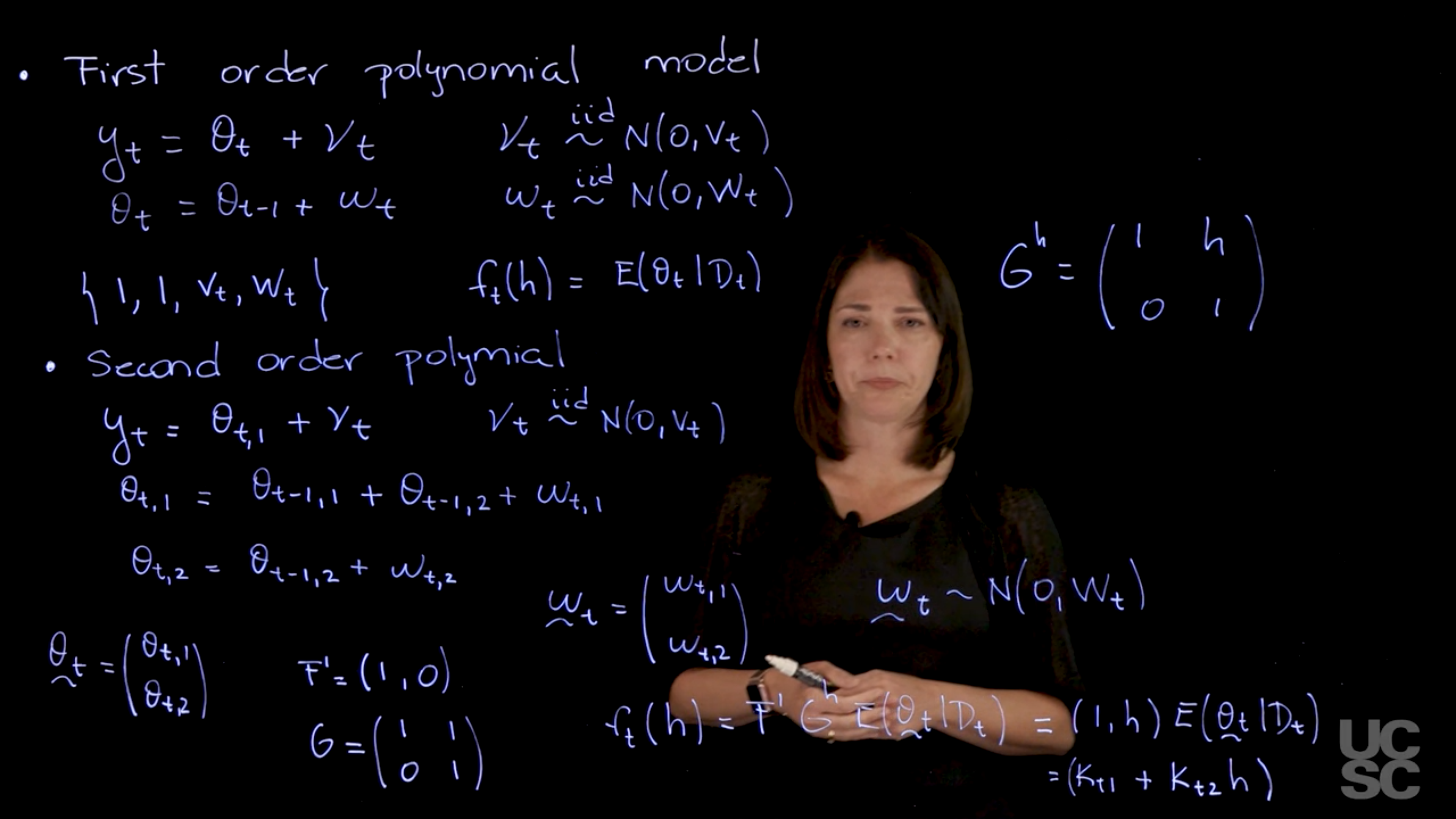
\begin{aligned} y_t &= \theta_t + \nu_t, \qquad & \nu_t & \overset{\text{iid}}{\sim} \mathcal{N}(0, V_t) \\ \theta_t &= \theta_{t-1} + \omega_t, \qquad & \omega_t & \overset{\text{iid}}{\sim} \mathcal{N}(0, W_t) \\ &\{1,1,v_t,W_t\} && \text{(short form)} \\ f_t(h) &= \mathbb{E}[\theta_t \mid \mathcal{D}_t] && \text{(forecast fn)} \\ \end{aligned} \tag{97.13}
In the observation equation, \theta_{t} is the level of the series at time t and \nu_t is the observation error. In the evolution equation we see the mean for this parameter changing over time as a random walk or a local constant mean with evolution noise \omega_t.
(West and Harrison 2013, sec. 2.1) gives the following representation of the model:
It is useful to think of \theta_t as a smooth function of time \theta(t) with an associated Taylor series representation
\theta(t + \delta t) = \theta(t) + \text{higher-order terms} \tag{97.14}
where the higher-order terms are assumed to be zero-mean noise. This is a very important point, because it means that we are not trying to model the higher-order terms explicitly, but rather we are assuming that they are just noise.
with the model simply describing the higher-order terms as zero-mean noise.
This is the genesis of the first-order polynomial DLM: the level model is a locally constant (first-order polynomial) proxy for the underlying evolution.·
We can write it down in short form with the following quadruple/
\{1, 1, V_t, W_t\} \qquad f_t(h) = \mathbb{E}[\theta_t \mid \mathcal{D}_t] = k_t \ \forall h>0 \tag{97.15}
Next we can write the forecast function f_t(h) of this model using the representation we gave in Equation 97.15.
Again, we’re going to have something of the form F transposed G to the power of h and then the expected value of that \theta_t given \mathcal{D}_t. F is 1, G is 1, therefore I’m going to end up having just expected value of \theta_t given \mathcal{D}_t.
Which depending on the data that you have is you’re just going to have something that is a value that depends on t and it doesn’t depend on h. What this model is telling you is that the forecast function, how you expect to see future values of the series h steps ahead is something that looks like the level that you estimated at time t.
(West and Harrison 2013, secs. 7.1–7.2) gives a detailed analysis of this model.
Now we want to create a model in which captures things that has a linear trend either increasing or decreasing. To do thus we need to have two components in our parameter vector of the state vector. For this we will need two components in our parameter vector of the state vector1.
So we have again something that looks like in my observation equation. I’m going to have, I’m going to call it say \theta_{t,1} \sim \mathcal{N}(v_t), and then I’m going to have say \theta_{t,1} is going to be of the form to \theta_{t-1,1} and there is another component here. The other component enters this equation plus let’s call this \theta_{t-1,2}. And then I have finally also I need an evolution for the second component of the process which is going to be again having a random walk type of behavior.
\begin{aligned} y_t &= \theta_{t,1} + \nu_t \quad &\nu_t &\overset{\text{iid}}{\sim} \mathcal{N}(0, v_t) \\ \theta_{t,1} &= \theta_{t-1,1} + \theta_{t-1,2} + \omega_{t,1} \qquad &\omega_{t,1} &\overset{\text{iid}}{\sim} \mathcal{N}(0, w_{t,11}) \\ \theta_{t,2} &= \theta_{t-1,2} + \omega_{t,2} \qquad &\omega_{t,2} &\overset{\text{iid}}{\sim} \mathcal{N}(0, w_{t,22}) \end{aligned} \tag{97.16}
So there are different ways in which you can interpret this two parameters but essentially:
Next we should summarize this model using the familiar short form DLM representation, which requires a bit of creative algebra.
\mathbf{\theta}_t = (\theta_{t,1}, \theta_{t,2}) \qquad \{\mathbf{F}, \mathbf{G}, V_t, \mathbf{W}_t\}
First we collect the two variances for the evolution two components into the vector \utilde{w}_t and then assume that this w_t is Normal. Now this is a bi-variate normal.
\utilde{\omega}_t = (\omega_{t,1},\omega_{t,2})' \qquad \utilde{\omega}_t \sim \mathcal{N}(0,W_t)
So what would be my F and my G in this model? So again my theta vector has two components, thus my G, so my F is going to be a two dimensional. We can write down F transposed as the only component that appears at this level is the first component of the vector. I’m going to have 1 and then a zero for F transposed. c.f. Equation 97.17 And then my G here if you think about writing down \theta_t times G say the t-1 + \omega_t. Then you have that you’re G is going to have this form.
\begin{aligned} \mathbf{F} &= (1,0)' & V_t &= v_t \\ \mathbf{G} &= \begin{pmatrix} 1 & h \\ 0 & 1 \end{pmatrix} & \mathbf{W}_t &= \begin{pmatrix} w_{t,11} & 0 \\ 0 & w_{t,22} \end{pmatrix} \end{aligned} \tag{97.17}
this is the form from the video \begin{aligned} \mathbf{F} &= (1,0)' & V_t &= v_t \\ \mathbf{G} &= \begin{pmatrix} 1 & h \\ 0 & 1 \end{pmatrix} & \mathbf{W}_t &= \begin{pmatrix} w_{t,11} & w_{t,12} \\ w_{t,21} & w_{t,22} \end{pmatrix} \end{aligned} \tag{97.18}
this is the more general form from the handout. Note that in this case we have w_{t,12}=w_{t,21} so there is just one extra parameter.
The lesson videos and the handouts differ in the form \mathbf{W}_t. In the lecture we assumed zero covariance but in the handout the covariance was snuck in. This gives us a slightly more general model. The covariance though is symmetric so we get an extra parameter we need to infer and include in the prior. Anyhow I kept the more general form, though in most cases we will keep the off diagonal terms at zero.
So for the first component, I have past values of both components. That’s why I have a 1 and 1 here for the second component I only have the past value of the second component. So there is a zero and a 1. So this tells me what is the structure of this second order polynomial. If I think about how to obtain the forecast function for this second order polynomial is going to be very similar to what we did before. So you can write it down as F transposed G to the power of h, expected value of theta t given Dt. Now the expected value is going to be vector also with two components because theta_t is a two dimensional vector. The structure here if you look at what G is G to the power of h going to be a matrix, that is going to look like 1, h, 0 1. When you multiply that matrix time this times this F what you’re going to end up having is something that looks like 1 h times this expected value of theta t given Dt. So I can think of two components here, so this gives you a constant on h, this part is not going to depend on h. So I can write this down as k t 11 component multiplied by 1 and then I have another constant, multiplied by h. So you can see what happens now is that your forecast function has the form of a linear polynomial. So it’s just a linear function on the number of steps ahead. The slope and the intercept related to that linear function are going to depend on the expected value of, theta_t given the all the information I have up to time t. But essentially is a way to model linear trends. So this is what happens with the second order polynomial model.
As we included linear trends and constant values in the forecast function, we may want to also incorporate other kinds of trends, polynomial trends in the model. So you may want to have a quadratic form, the forecast function or a cubic forecast function as a function of h.
\theta_t = (\theta_{t,1}, \theta_{t,2})' \qquad \mathbf{G} = \mathbf{J}_2(1) \qquad \mathbf{E}_2 = (1, 0)'
\mathbf{G^h} = \begin{pmatrix} 1 & h \\ 0 & 1 \end{pmatrix}
\begin{aligned} f_t(h) &= F' G^h \mathbb{E}[\theta_t \mid \mathcal{D}_t] \\ &= (1,h) \mathbb{E}[\theta_{t}\mid D_t] \\ &= (1,h)(K_{t,0}, K_{t,1})' \\ &= (K_{t,0} + K_{t,1} h) \end{aligned} \tag{97.19}
\begin{aligned} \mathbf{G^h} &= \begin{pmatrix} 1 & h \\ 0 & 1 \end{pmatrix} \end{aligned} \tag{97.20}
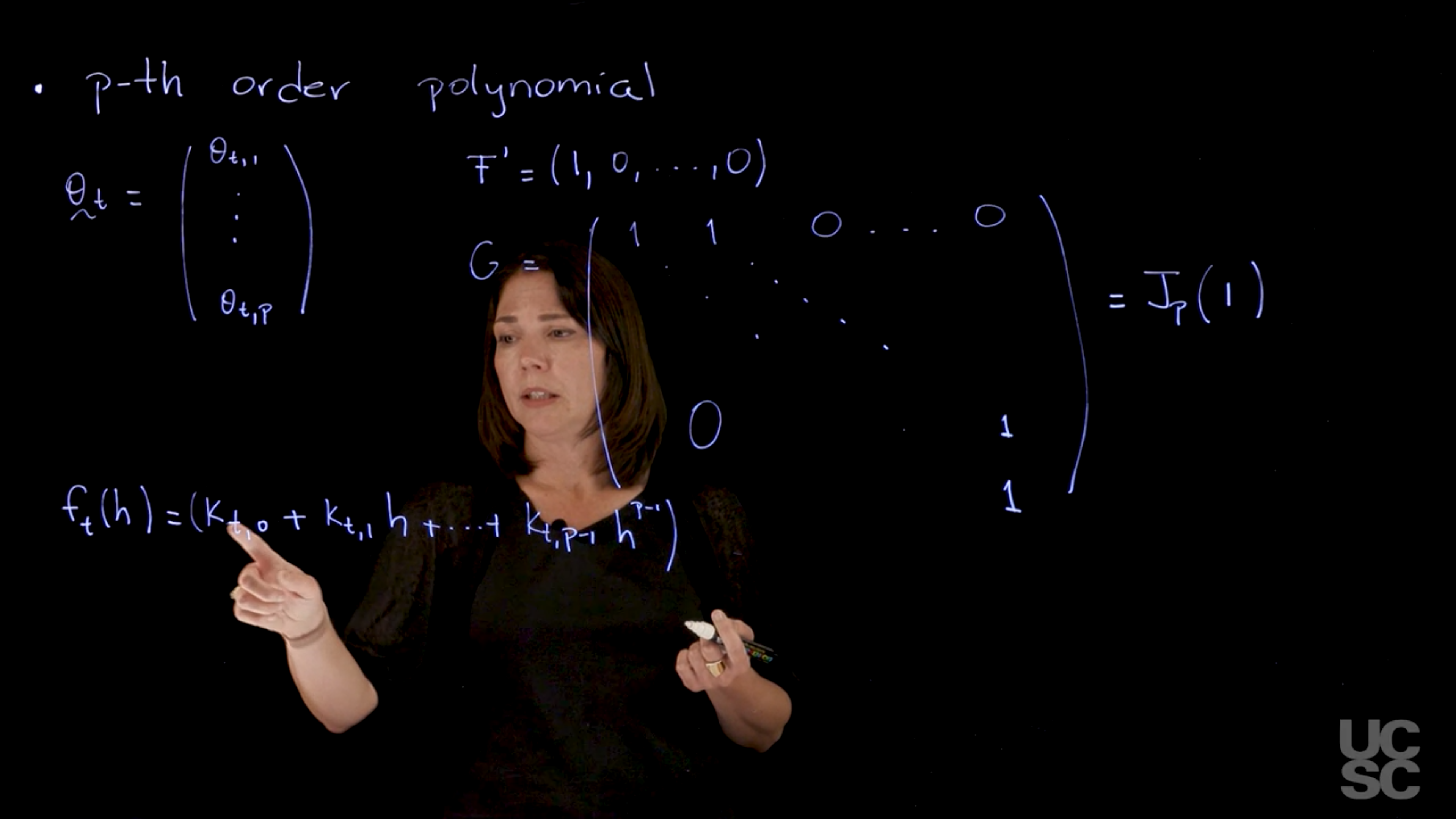
We can consider a so called p-th order polynomial model. This model will have a state-space vector of dimension p and a polynomial of order p − 1 forecast function on h. The model can be written as
\{E_p, J_p(1), v_t, W_t\}
with F_t = E_p = (1, 0, \ldots, 0)′ and G_t = J_p(1), with
J_p(1) = \begin{pmatrix} 1 & 1 & 0 & \cdots & 0 & 0 \\ 0 & 1 & 1 & \cdots & 0 & 0 \\ 0 & 0 & 1 & \cdots & 0 & 0 \\ \vdots & \vdots & \vdots & \ddots & \vdots \\ 0 & 0 & 0 & \cdots & 1 & 1 \\ 0 & 0 & 0 & \cdots & 0 & 1 \end{pmatrix} \tag{97.21}
The forecast function is given by f_t(k) = a_{t_0} + a_{t_1}k + \ldots + a_{t_{n-1}} k^{n-1} \qquad k \in \mathbb{N} \tag{97.22}
where a_{t_i} are the coefficients of the polynomial and k is the number of steps ahead we need in our forecast. There is also an alternative parameterization of this model that leads to the same algebraic form of the forecast function given by \{Ep, Lp, vt, W t\}, with
L_p = \begin{pmatrix} 1 & 1 & 1 & \cdots & 1 & 1 \\ 0 & 1 & 1 & \cdots & 1 & 1 \\ 0 & 0 & 1 & \cdots & 1 & 1 \\ \vdots & \vdots & \vdots & \ddots & \vdots \\ 0 & 0 & 0 & \cdots & 1 & 1 \\ 0 & 0 & 0 & \cdots & 0 & 1 \end{pmatrix} \tag{97.23}
And in this type of model, the forecast function is going to have order p-1. So the parameter vector is going to have dimension p. So you’re going to have \theta_t = \theta_{t1:p}.
The observation operator F is just a constant and if we write it as a row vector we get F' as a p-dimensional vector with the one in the first entry and zeros everywhere else.
The dynamics matrix G may be written using either a J Jordan form Equation 97.21 or as a triangular form Equation 97.23. These result in different parameterization of this model and we will talk a little bit about this.
In the Equation 97.21 we have a matrix with ones on the diagonal and the super diagonal, the matrix is needs to be p \times p i.e. with dimension p to be compatible with the dimension of the hidden state vector \theta. So this matrix G is what we call a Jordan block of dimension p of 1. So here 1 is the number that appears in the diagonal. And then I have a p I_p matrix, I have ones in the upper diagonal part. So this is the form of the model, so once again I have the F the G, and the W_t. I have my model.
The forecast function in this case again can be written as F' G^h \mathbb{E}[\theta_t \mid \mathcal{D}_t]. And when you simplify times expected value of \theta_t, given D_t. Once you simplify those functions you get something that is a polynomial of order p-1 in h. So I just can write this down as k_t + k_{t,1} h + k_{t, p-1} h^{p-1}, so that’s my forecast function.
There is an alternative parameterization of this model that has the same F and the same algebraic form of the forecast function, the same form of the forecast function. But instead of using Equation 97.21 form of the G matrix, it has a Equation 97.23 form that has ones in the diagonal and ones everywhere above the diagonal. So it’s an upper triangular matrix with ones in the diagonal and above the diagonal. That’s a different parameterization of the same model but it leads to the same general form of the forecast function just with a different parameterization.
So again, we can consider the way you think about these models?
Note that the third order polynomial model is covered in
I will begin describing the structure of a particular class of models now, the polynomial trend models. These are models that are useful to describe linear trends or polynomial trends in your time series. So if you have a data set, where you have an increasing trend, or a decreasing trend, you would use one of those components in your model.
We will begin with the first order polynomial model, which we have already described. It’s the one that has y_t is a single parameter, I’m going to call it just \theta_t + \nu_t. And then a random walk evolution for that single parameter, so that’s the mean level of the series. And then we assume that it changes as a random walk, so this is the first order polynomial model.
So in general, I’m going to begin with the first order polynomial model, which we have already described. It’s the one that has y_t is a single parameter, I’m going to call it just \theta_t + \nu_t. And then a random walk evolution for that single parameters, so that’s the mean level of the series. And then we assume that it changes As a random walk, so this is the first order polynomial model. In this model if I want to write it down in short form I would have a quadruple that looks like this. So the F here that goes F transposed times the parameter vector in this case we have a scalar vector, scalar parameter. It’s going to be 1 my G that goes next to the state of t-1 is going to also be 1. And then I have vt and Wt here. So this fully defines my model if I think about the forecast function of this model using the representation we had before. Again, we’re going to have something of the form F'G^h and then the expected value of that \theta_t | \mathcal{D}_t. F is 1, G is 1, therefore I’m going to end up having just expected value of \theta_t | \mathcal{D}_t. Which depending on the data that you have is you’re just going to have something that is a value that depends on t and it doesn’t depend on h.
What this model is telling you is that the forecast function, how you expect to see future values of the series h steps ahead is something that looks like the level that you estimated at time t.
So that’s the forecast function, you is a first order is a zero order polynomial is a constant on h and it’s called the first order polynomial model.
In the case of a second order polynomial We are going to now think about about a model in which we want to capture things that are not a constant over time but may have an increasing or decreasing linear trend. In this case we’re going to need two components in your parameter vector in the state vector.
So we have again something that looks like in my observation equation. I’m going to have, I’m going to call it say theta{t,1} Normal vt, and then I’m going to have say theta_{t,1} is going to be of the form to theta_{t-1,1} and there is another component here. The other component enters this equation plus let’s call this And then I have finally also I need an evolution for the second component of the process which is going to be again having a random walk type of behavior. So there is different ways in which you can interpret this two parameters but essentially one of them is related to the baseline level of the series the other one is related to the rate of change of the of the series. So if you think about the dlm representation again, these two components, I can collect into the vector wt. and then assume that this wt Is normal. Now this is a bivariate normal. So what would be my F and my G in this model? So again my theta vector has two components My G, so my F is going to be a two dimensional vectors. So I can write down F transposed as the only component that appears at this level is the first component of the vector. I’m going to have 1 and then a zero for F transposed. And then my G here if you think about writing down theta t times G say the t -1 +wt. Then you have that you’re G is going to have this form. So for the first component, I have past values of both components. That’s why I have a 1 and 1 here for the second component I only have the past value of the second component. So there is a zero and a 1. So this tells me what is the structure of this second order polynomial. If I think about how to obtain the forecast function for this second order polynomial is going to be very similar to what we did before. So you can write it down as F transposed G to the power of h, expected value of theta t given Dt. Now the expected value is going to be vector also with two components because theta_t is a two dimensional vector. The structure here if you look at what G is G to the power of h going to be a matrix, that is going to look like 1, h, 0 1. When you multiply that matrix time this times this F what you’re going to end up having is something that looks like 1 h times this expected value of theta t given Dt. So I can think of two components here, so this gives you a constant on h, this part is not going to depend on h. So I can write this down as k t 11 component multiplied by 1 and then I have another constant, multiplied by h. So you can see what happens now is that your forecast function has the form of a linear polynomial. So it’s just a linear function on the number of steps ahead. The slope and the intercept related to that linear function are going to depend on the expected value of, theta_t given the all the information I have up to time t. But essentially is a way to model linear trends. So this is what happens with the second order polynomial model.
As we included linear trends and constant values in the forecast function, we may want to also incorporate other kinds of trends, polynomial trends in the model. So you may want to have a quadratic form, the forecast function or a cubic forecast function as a function of h. So the all those can be incorporated using the general p-order polynomial model, so I will just describe the form of this model. And in this type of model, the forecast function is going to have order p-1. So your parameter vector is going to have dimension p. So you’re going to have theta_t theta t1 to tp. Your F matrix is going to be constant if I write it as a row vector. F transpose is going to be a p dimensional vector with the one in the first entry and zeros everywhere else. My G matrix is going to have this form and there is different parameterizations of this model and I will talk a little bit about this. But one way to parameterize the model is something that looks like this. So you have ones in the diagonal of the matrix, the matrix is going to be a p by p has to be the dimension of the p compatible with the dimension of the state vector. And then you have zeros’s below the diagonal above that set of ones that are also ones above the diagonal. So this matrix G is what we call a Jordan block of dimension p of 1. So here 1 is the number that appears in the diagonal. And then I have a p Ip matrix, I have ones in the upper diagonal part. So this is the form of the model, so once again I have the F the G, and the wt. I have my model. The forecast function in this case again can be written as F transposed G to the power of h. And when you simplify times expected value of theta_t, given Dt. Once you simplify those functions you get something that is a polynomial of order p-1 in h. So I just can write this down as kt constant.Plus kt1 h + kt p- 1, h to the p -1, so that’s my forecast function. There is an alternative parameterization of this model that has the same F and the same algebraic form of the forecast function, the same form of the forecast function. But instead of having this G matrix, it has a matrix that has ones in the diagonal and ones everywhere above the diagonal. So it’s an upper triangular matrix with ones in the diagonal and above the diagonal. That’s a different parameterization of the same model is going to have the same general form of the forecast function is a different parameterization. So again, you can consider the way you think about these models is you think what kind of forecast function I want to have for my future? What is the type of predictions that I expect to have in my model? And if they look like a linear trend, I use a second order polynomial. If it looks like a quadratic trend in the forecast then I would use 3rd order polynomial model representation.
\begin{aligned} y_t &= \mu_t + \nu_t, \qquad & \nu_t &\sim \mathcal{N}(0, v_t) \\ \mu_t &= \mu_{t-1} + \omega_t, \qquad & \omega_t &\sim \mathcal{N}(0, w_t) \end{aligned}
In this case, we have:
\theta_t = \mu_t \quad \forall t
F_t = 1 \quad \forall t \qquad G_t = 1 \quad \forall t
resulting in:
\{1, 1, v_t, w_t\} \qquad \text{(short notation)}
The forecast function is:
f_t(h) = E(\mu_t \mid \mathcal{D}_t) = k_t, \quad \forall h > 0.
\begin{aligned} y_t &= \theta_{t,1} + \nu_t, \quad &\nu_t &\sim \mathcal{N}(0, v_t) \\ \theta_{t,1} &= \theta_{t-1,1} + \theta_{t-1,2} + \omega_{t,1}, \qquad &\omega_{t,1} &\sim \mathcal{N}(0, w_{t,11}) \\ \theta_{t,2} &= \theta_{t-1,2} + \omega_{t,2}, \qquad &\omega_{t,2} &\sim \mathcal{N}(0, w_{t,22}), \end{aligned}
where we can also have:
\mathbb{C}ov(\theta_{t,1}, \theta_{t,2} ) = w_{t,12} = w_{t,21}
This can be written as a DLM with the state-space vector \theta_t = (\theta_{t,1}, \theta_{t,2})', and
\{\mathbf{F}, \mathbf{G}, v_t, \mathbf{W}_t\} \qquad \text{(short notation)}
with \mathbf{F} = (1, 0)' and
\mathbf{G} = \begin{pmatrix} 1 & 1 \\ 0 & 1 \end{pmatrix}, \quad \mathbf{W}_t = \begin{pmatrix} w_{t,11} & w_{t,12} \\ w_{t,21} & w_{t,22} \end{pmatrix}.
Note that
\mathbf{G}^2 = \begin{pmatrix} 1 & 2 \\ 0 & 1 \end{pmatrix}, \quad \mathbf{G}^h = \begin{pmatrix} 1 & h \\ 0 & 1 \end{pmatrix},
and so:
f_t(h) = (1, h) E(\mathbf{\theta}_t \mid \mathcal{D}_t) = (1, h) (k_{t,0}, k_{t,1})' = (k_{t,0} + h k_{t,1}).
Here \mathbf{G} = \mathbf{J}_2(1) (see below).
Also, we denote \mathbf{E}_2 = (1, 0)', and so the short notation for this model is
\{E_2, J_2(1), \cdot, \cdot\}
We can consider a p-th order polynomial model. This model will have a state-space vector of dimension p and a polynomial of order p-1 forecast function on h. The model can be written as
\{E_p, J_p(1), v_t, W_t\} \qquad \text{(short notation)}
with \mathbf{F}_t = \mathbf{E}_p = (1, 0, \dots, 0)' and \mathbf{G}_t = \mathbf{J}_p(1), with
\mathbf{J}_p(1) = \begin{pmatrix} 1 & 1 & 0 & \cdots & 0 & 0 & 0 \\ 0 & 1 & 1 & \cdots & 0 & 0 & 0 \\ \vdots & \vdots & \ddots & \ddots & & \vdots \\ 0 & 0 & 0 & \cdots & 0 & 1 & 1 \\ 0 & 0 & 0 & \cdots & 0 & 0 & 1 \end{pmatrix}.
The forecast function is given by
f_t(h) = k_{t,0} + k_{t,1} h + \dots + k_{t,p-1} h^{p-1}.
There is also an alternative parameterization of this model that leads to the same algebraic form of the forecast function, given by \{E_p, L_p, v_t, W_t\}, with
L_p = \begin{pmatrix} 1 & 1 & 1 & \cdots & 1 \\ 0 & 1 & 1 & \cdots & 1 \\ \vdots & \vdots & \ddots & \ddots & \vdots \\ 0 & 0 & 0 & \cdots & 1 \end{pmatrix}.
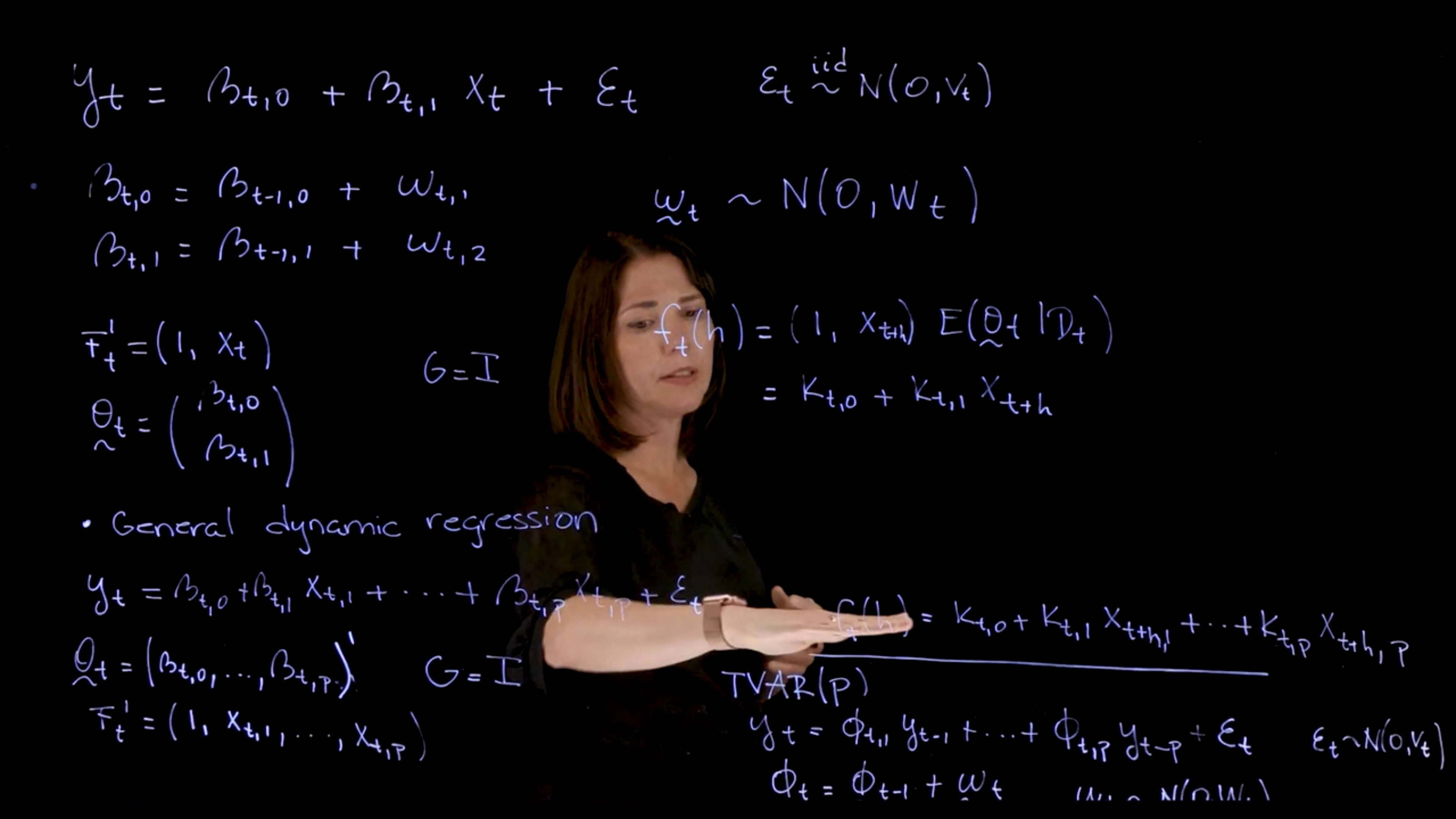
\begin{aligned} y_t &= \beta_{t,0} + \beta_{t,1}x_t + ν_t \\ \beta_{t,0} &= \beta_{t−1,0} + \omega_{t,0} \\ \beta_{t,1} &= \beta_{t−1,1} + \omega_{t,1} \end{aligned} \tag{97.24}
and so \theta_t = (\beta_t,0, \beta_{t,1})′, F_t = (1, x_t)′ and G = I_2.
This results in a forecast function of the form
f_t(h) = k_{t,0} + k_{t,1}x_{t+h} \tag{97.25}
where k_{t,0} = \mathbb{E}[\beta_{t,0} \mid \mathcal{D}_t] and k_{t,1} = \mathbb{E}[\beta_{t,1} \mid \mathcal{D}_t].
\begin{aligned} y_t &= \beta_{t,0} + \beta_{t,1}x_{t,1} + \ldots \beta_{t,M} x_{t,M} + ν_t \\ \beta_{t,m} &= \beta_{t−1,m} + \omega_{t,m,} & m = 0 : M. \end{aligned} \tag{97.26}
Then, \theta = (\beta_t,0, \ldots , \beta_{t,M} )′, F_t = (1, x_{t,1}, \ldots , x_{t,M} )′ and G = I_M . The forecast function is given by
f_t(h) = k_{t,0} + k_{t,1}x_{t+h,1} + \ldots + k_{t+h,M}x_{t+h,M} \tag{97.27}
A particular case is of dynamic regressions is the case of time-varying auto-regressions (TVAR) with
\begin{aligned} y_t &= \varphi_{t,1}y_{t−1} + \varphi_{t,2}y_{t−2} + \ldots + \varphi_{t,p} y_{t−p} + ν_t,\\ \varphi_{t,m} &= \varphi_{t−1,m} + \omega_{t,m,} & m = 1 : p \end{aligned} \tag{97.28}
There is a paper (Raquel Prado, Huerta, and West 2000) on TVAR models that is a good reference for this model.
In regression models, we may also have additional covariates that are also measured sequentially over time. We may want to regress the y_t time series and see what relationships they have with other covariates that are also measured over time. The simplest possible case is the dynamic simple regression model. In this case, I can write down. I have a single covariate, that covariate is X_t that is observed here, and then I have the usual. In this case, I have an intercept and a slope, and this is representing my simple linear regression. It’s just the regression where both the intercept and the slope are time-varying. I can define the variation. I need to specify what’s the evolution of the two components, and we are going to use this random walk. We could use other structures, but again, in the normal linear case, we are going to be using these evolution equations. Then I collect here my W’s as a single vector. The \omega_t is going to have the two components in here. These are normally distributed zero and variance covariance matrix W_t, that is a two-by-two matrix. This is the case of the simple regression model. In the case of this model, we have F now is time-varying. This is going to change depending on the value of X_t. I can write Ft transpose as one and X_t. My Theta vector. Again, if I think about what it is, is just Beta t, 0 Beta t, 1. I have those two components.
The G matrix is going to be the identity, and you can see that essentially the first component is related to the first component in t minus one, and the second component at time t is related to the second component at time t minus 1. So the identity matrix will be the G. Therefore, if I think about my forecast function in the simple linear regression case, this is going to be my F transpose, which is 1 xt times the G, the G is the identity, times the expected value of Theta t, given Dt. For the expected value of Theta t given Dt, This is a two-dimensional vector, so I’m going to have components in there. I can write this down as K_t0 plus K_t1 Xt. We can see that the forecast function is again has that form that depends on that covariate at the time. This should be t plus h because we are evaluating this at t plus h. You need to have the covariate evaluated at t plus h here.
In the case of general dynamic regression model, we’re going to have a set of covariates. We can have, let’s say k of those covariates or p of those covariates, X_t1. This is my observation equation. Instead of having a single covariate, now I’m going to have p of them. I’m going to have coefficients that go with each of those and I may have the Beta t0 coefficient. My G matrix now, if I think about my parameter vector is just p plus 1 dimensional, p plus 1. Yeah, so that I have the 0 and then the p values, so is a p plus 1 vector. Then my G is the identity. My F_t is going to be a vector, is also p plus 1 dimension. The first entry is one, the second is X_t1 X_tp. My forecast function is going to be similar to this, but now we are going to have more than one covariate, so we end up with a forecast function that has this form, p. This is the case for the dynamic regression.
In the case of dynamic regression, we can also have a time-varying autoregressive process. This is a particular case of dynamic regression where the covariates are just past values of the time series itself. In this case, we can think about the observation equation as being a linear combination of past values of the time series. One particular example of dynamic regression model is the case of a time-varying autoregressive process. This brings us back to those autoregressive processes that we were discussing earlier in the course. When you you’re regressing each of the X’s correspond to pass values, you have a regression model that we call a time-varying ARP. In this case, your observation equation is going to have the AR coefficients, but the AR coefficients are going to be varying over time. If we assume that we put all the coefficients together and have a random walk evolution equation for those. If I said, I call Phi_t the vector that contains all the components with all the coefficients from one to p, then I can now define this evolution equation. Then my Omega_t here is a p-dimensional vector, and I have Omega t, normal zero, WT, and my epsilon t normal 0 vt.
This defines a time-varying AR. It’s the same structure that we had before. The only difference is my covariates are just past values of the time series. Therefore my forecast function for the time-varying AR is going to have this form where every_thing is going to depend on past values of the time series. We will study this model in particular and make connections with the AR that we studied earlier in the class.
\begin{aligned} y_t &= \beta_{t,0} + \beta_{t,1} x_t + \nu_t \\ \beta_{t,0} &= \beta_{t-1,0} + \omega_{t,0} \\ \beta_{t,1} &= \beta_{t-1,1} + \omega_{t,1} \end{aligned}
Thus:
\theta_t = (\beta_{t,0}, \beta_{t,1})'
F_t = (1, x_t)'
and
G = I_2
This results in a forecast function of the form
f_t(h) = k_{t,0} + k_{t,1} x_{t+h}.
\begin{aligned} y_t &= \beta_{t,0} + \beta_{t,1} x_{t,1} + \dots + \beta_{t,M} x_{t,M} + \nu_t \\ \beta_{t,m} &= \beta_{t-1,m} + \omega_{t,m}, \quad &m = 0:M. \end{aligned} \tag{97.29}
Then,
\theta_t = (\beta_{t,0}, \dots, \beta_{t,M})',
\mathbf{F}_t = (1, x_{t,1}, \dots, x_{t,M})' and
\mathbf{G} = \mathbf{I}_M.
The forecast function is given by:
f_t(h) = k_{t,0} + k_{t,1} x_{t+h,1} + \dots + k_{t,M} x_{t+h,M}. \tag{97.30}
A particular case of dynamic regressions is the case of time-varying autoregressive (TVAR) with
\begin{aligned} y_t &= \phi_{t,1} y_{t-1} + \phi_{t,2} y_{t-2} + \dots + \phi_{t,p} y_{t-p} + \nu_t \\ \phi_{t,m} &= \phi_{t-1,m} + \omega_{t,m}, \quad m = 1:p. \end{aligned}
We can use the superposition principle to build models that have different kinds of components. The main idea is to think about what is the general structure we want for the forecast function and then isolate the different components of the forecast function and think about the classes of dynamic linear models that are represented in each of those components. Each of those components has a class and then we can build the general dynamic linear model with all those pieces together using this principle.
Two references for the Superposition principle are
In the first the author state:
Conditional independence also features strongly in initial model building and in choosing an appropriate parametrization. For example, the linear superposition principle states that any linear combination of deterministic linear models is a linear model. This extends to a normal linear superposition principle:
Any linear combination of independent normal DLMs is a normal DLM. - > – (West and Harrison 2013, sec. 3.1 p. 98)
We will illustrate how to do that with an example:
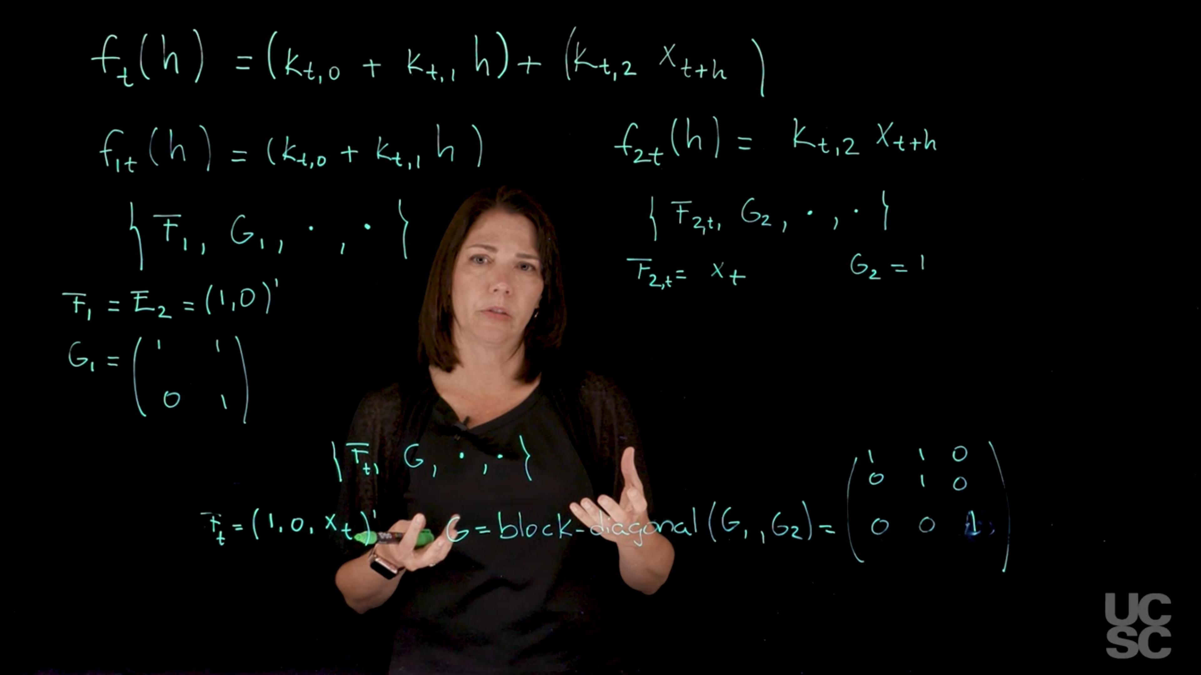
Let’s say that we want to create a model here with a forecast function that has a linear trend component. Let’s say we have a linear function as a function of the number of steps ahead that you want to consider. Then suppose you also have a covariate here that you want to include in your model as a regression component. f_t(h) = \underbrace{(k_{t,0} + k_{t,1}\; h)}_{\text{linear trend component}} + \underbrace{(k_{t,2}\; x_{t+h})}_{\text{regression component}} \tag{97.31}
where:
When we look at the forecast function, we can isolate a linear trend and a regression components as indicated. Each of these can be set in terms of two forecast functions]{.mark}. I’m going to call the forecast function f_{1,t}(h), this is just the first piece.
\begin{aligned} f_t(h) &= f_{1,t}(h) + f_{2,t}(h) \\ f_{1,t}(h) &= k_{t,0} + k_{t,1} & \text{(linear trend component)} \\ f_{2,t}(h) &= k_{t,2}x_{t+h} & \text{(regression component)} \end{aligned} \tag{97.32}
We know how to represent forecast function f_{1,t} and f_{2,t} in terms of dynamic linear models.
For the linear trend component, f_{1,t}(h) , we have a 2-dimensional state vector, \theta_t = (\theta_{t,1}, \theta_{t,2})', which yields the following DLM shortform:
\{F_1, G_1, \cdot, \cdot\} \qquad \text{(short notation)} \tag{97.33}
F_{1} = E_2 = (1, 0)' \tag{97.34}
G_{1} = \begin{pmatrix} 1 & 1 \\ 0 & 1 \end{pmatrix} \tag{97.35}
for the regression component f_{2,t}(h) we have the following DLM representation:
\{F_2,t, G_2, \cdot, \cdot\} \qquad \text{(short notation)} \tag{97.36}
where we have F_{2t} is X_t and my G is simply going to be 1. This is a one-dimensional vector in terms of the state parameter vector.
F_{2,t} = x_{t+h} \tag{97.37}
G_{2} = 1 \tag{97.38}
Once we have these, we can assemble them into our final model. \{F_t, G, \cdot, \cdot\}
We care more about F, G, and less about the observational variance and some covariance also for the system where the
F is going to be an F that has, you just concatenate the two Fs. You’re going to get 1, 0 and then you’re going to put the next component here. Again, this one is dependent on time because this component is time dependent and
The model with forecast function f_t(h) above is a model with a 3-dimensional state vector with
F_t = (F_1', F_{2,t})' = (1, 0, x_t)'
Then the G, you can create it just taking a block diagonal structure by concatenating G_1 and G_2. though formally there must be a better term for this operation.
G = \text{blockdiag}[G_1, G_2] = \begin{pmatrix} 1 & 1 & 0 \\ 0 & 1 & 0 \\ 0 & 0 & 1 \end{pmatrix}.
This gives us the full G dynamics matrix for the model. A model with this F_t and this G that is constant over time will give us this particular forecast function Equation 97.31 we started with.
We used the superposition principle to build this model. If we need additional components, we will learn how to incorporate seasonal components, regression components, trend components. One can build a fairly sophisticated model with different structures into this particular model using the superposition principle.
We can use the superposition principle to build models that have different kinds of components. The main idea is to think about what is the general structure we want for the forecast function and then isolate the different components of the forecast function and think about the classes of dynamic linear models that are represented in each of those components. Each of those components has a class and then we can build the general dynamic linear model with all those pieces together using this principle. I will illustrate how to do that with an example. Let’s say that you want to create a model here with a forecast function that has a linear trend component. Let’s say we have a linear function as a function of the number of steps ahead that you want to consider. Then suppose you also have a covariate here that you want to include in your model as a regression component. Let’s say we have a K_t2 and then we have X_t plus h, this is my covariate. Again, the k’s here are just constants, as of constants in terms of h, they are dependent on time here. This is the general structure we want to have for the forecast function. Now you can see that when I look at the forecast function, I can isolate here and separate these two components. I have a component that looks like a linear trend and then I have a component that is a regression component. Each of this can be set in terms of two forecast functions. I’m going to call the forecast function F_1t h, this is just the first piece. Then I have my second piece here. I’m going to call it F_2t, is just this piece here with the regression component. We know how to represent this forecast function in terms of a dynamic linear model. I can write down a model that has an F, G, and some V, and some W that I’m going to just leave here and not specify them explicitly because the important components for the structure of the model are the F and the G. If you’ll recall the F in the case of a forecast function with a linear trend like this, is just my E_2 vector, which is a two-dimensional vector. The first entry is one, and the second one is a zero. Then the G in this case is just this upper triangular matrix that has 1, 1 in the first row and 0, 1 in the second one. Remember, in this case we have a two-dimensional state vector where one of the components in the vector is telling me information about the level of the time series, the other component is telling me about the rate of change in that level. This is a representation that corresponds to this forecast function. For this other forecast function, we have a single covariate, it’s just a regression and I can represent these in terms of an F_2, G_2, and then some observational variance and some system variance here in the case of a single covariate and this one depends on t. We have F_2t is X_t and my G here is simply going to be one. This is a one-dimensional vector in terms of the state parameter vector. We have a single state vector and it’s just going to tell me about the changes, the coefficient that goes with the X_t covariate. Once I have these, I can create my final model and I’m going to just say that my final model is F, G, and then I have some observational variance and some covariance also for the system where the F is going to be an F that has, you just concatenate the two Fs. You’re going to get 1, 0 and then you’re going to put the next component here. Again, this one is dependent on time because this component is time dependent and then the G, you can create it just taking a block diagonal structure, G_1 and G_2. You just put together, the first one is 1, 1, 0, 1 and then I concatenate this one as a block diagonal. This should be one. This gives me the full G function for the model. Now a model with this F_t and this G that is constant over time will give me this particular forecast function. I’m using the superposition principle to build this model. If you want additional components, we will learn how to incorporate seasonal components, regression components, trend components. You can build a fairly sophisticated model with different structures into this particular model using the superposition principle.
You can build dynamic models with different components, for example, a trend component plus a regression component, by using the principle of superposition. The idea is to think about the general form of the forecast function you want to have for prediction. You then write that forecast function as a sum of different components where each component corresponds to a class of DLM with its own state-space representation. The final DLM can then be written by combining the pieces of the different components.
For example, suppose you are interested in a model with a forecast function that includes a linear polynomial trend and a single covariate x_t, i.e.,
f_t(h) = k_{t,0} + k_{t,1}h + k_{t,3}x_{t+h}.
This forecast function can be written as f_t(h) = f_{1,t}(h) + f_{2,t}(h), with
f_{1,t}(h) = (k_{t,0} + k_{t,1}h), \quad f_{2,t}(h) = k_{t,3}x_{t+h}.
The first component in the forecast function corresponds to a model with a 2-dimensional state vector, F_{1,t} = F_1 = (1, 0)',
G_{1,t} = G_1 = \begin{pmatrix} 1 & 1 \\ 0 & 1 \end{pmatrix}.
The second component corresponds to a model with a 1-dimensional state vector, F_{2,t} = x_t, G_{2,t} = G_2 = 1.
The model with forecast function f_t(h) above is a model with a 3-dimensional state vector with F_t = (F_1', F_{2,t})' = (1, 0, x_t)' and
G_t = \text{blockdiag}[G_1, G_2] = \begin{pmatrix} 1 & 1 & 0 \\ 0 & 1 & 0 \\ 0 & 0 & 1 \end{pmatrix}.
The general case wasn’t covered in the video and we didn’t have a proper statement of the superposition principle. However, in Important 97.1 I extracted the statement of the principle above. This statement clarifies that the principle arises via conditional independence, a tool we also used extensively in the previous course on mixture models. Now let us consider the general case from the handout.
Assume that you have a time series process y_t with a forecast function
f_t(h) = \sum_{i=1}^{m} f_{i,t}(h),
where each f_{i,t}(h) is the forecast function of a DLM with representation \{F_{i,t}, G_{i,t}, v_{i,t}, W_{i,t}\}.
Then, f_t(h) has a DLM representation \{F_t, G_t, v_t, W_t\} with
F_t = (F_{1,t}', F_{2,t}', \dots, F_{m,t}')',
G_t = \text{blockdiag}[G_{1,t}, \dots, G_{m,t}],
v_t = \sum_{i=1}^{m} v_{i,t},
and
W_t = \text{blockdiag}[W_{1,t}, \dots, W_{m,t}].
the state makes it’s appearance↩︎