---
title: "Appendix: Continuous Distributions"
---
Following a subjective view of distribution, which is more amenable to reinterpretation I use an indicator function to place restrictions on the range of parameter of the PDF.
```{r include=FALSE}
#| label: A03-1
# Necessary for using dvisvgm on macOS
# See https://www.andrewheiss.com/blog/2021/08/27/tikz-knitr-html-svg-fun/
Sys.setenv(LIBGS = "/usr/local/share/ghostscript/9.53.3/lib/libgs.dylib.9.53")
font_opts <- list(dvisvgm.opts = "--font-format=woff")
```
## The Continuous Uniform {#sec-continuous-uniform}
### Stories
::: {.callout-note}
#### Discrete Uniform Finite set Parametrization
:::
$$
X \sim U[\alpha,\beta]
$$ {#eq-cont-uniform-rv}
### Moments
$$
\mathbb{E}[X]=\frac{(\alpha+\beta)}{2}
$$ {#eq-cont-uniform-expectation}
$$
\mathbb{V}ar[X]=\frac{(\beta-\alpha)^2}{12}
$$ {#eq-cont-uniform-variance}
### Probability mass function (PDF)
$$
f(x)= \frac{1}{\alpha-\beta} \mathbb{I}_{\{\alpha \le x \le \beta\}}(x)
$$ {#eq-cont-uniform-PDF}
### Cumulative distribution function (CDF)
$$
F(x\mid \alpha,\beta)=\begin{cases}
0, & \text{if }x < \alpha \\
\frac{x-\alpha}{\beta-\alpha}, & \text{if } x\in [\alpha,\beta]\\
1, & \text{if } x > \beta
\end{cases}
$$ {#eq-cont-uniform-CDF}
### Prior
Since a number of families have the uniform as a special case we can use them as priors when we want a uniform prior:
$Normal(0,1)= Beta(1,1)$
## The Beta Distribution {#sec-the-beta-distribution}
\index{distribution!beta}
### Story
The Beta distribution is used for random variables which take on values between 0 and 1. For this reason (and other reasons we will see later in the course), the Beta distribution is commonly used to model probabilities.
$$
X \sim Beta(\alpha, \beta)
$$ {#eq-beta-rv}
### PDF & CDF
$$
f(x \mid \alpha, \beta) = \frac{\Gamma(\alpha + \beta)}{\Gamma(\alpha)\Gamma(\beta)} x^{\alpha−1}(1 − x)^{\beta−1}\mathbb{I}_{x\in(0,1)}\mathbb{I}_{\alpha\in\mathbb{R}^+}\mathbb{I}_{\beta\in\mathbb{R}^+} \qquad \text{(PDF)}
$$ {#eq-beta-pdf}
$$
\begin{aligned}
& F(x \mid \alpha,\beta) &= I_x(\alpha,\beta) && \text{(CDF)} \\
\text{where } & I_w(u,v) & &&\text{ is the regularized beta function: } \\
& I_w(u,v) &= \frac{B(w; u, v)}{B(u,v)} \\
\text{where }& B(w; u,v) &=\int_{0}^{w}t^{u-1}(1-t)^{v-1}\mathrm{d}t && \text{ is the incomplete beta function }\\
\text{and } & B(u,v)& && \text{ is the (complete) beta function}
\end{aligned}
$$ {#eq-beta-cdf}
### Moments
$$
\mathbb{E}[X] = \frac{\alpha}{\alpha + \beta} \qquad (\text{expectation})
$$ {#eq-beta-expectation}
$$
\mathbb{V}ar[X] = \frac{\alpha\beta}{(\alpha + \beta)^2 (\alpha + \beta + 1)} \qquad (\text{variance})
$$ {#eq-beta-variance}
$$
\mathbb{M}_X(t) = 1+ \sum^\infty_{i=1} \left ( {\prod^\infty_{j=0} \frac{\alpha+j}{\alpha + \beta + j} } \right ) \frac{t^i}{i!}
$$ {#eq-beta-mgf}
where $\Gamma(·)$ is the **Gamma function** introduced with the gamma distribution.
Note also that $\alpha > 0$ and $\beta > 0$.
### Relations
The standard $Uniform(0, 1)$ distribution is a special case of the beta distribution with $\alpha = \beta = 1$.
$$
Uniform(0, 1) = Beta(1,1)
$$ {#eq-uniform-as-beta}
### As a prior
The Beta distribution is often used as a prior for parameters that are **probabilities**,since it takes values from 0 and 1.
During prior elicitation the parameters can be set using
1. the mean: $\alpha \over \alpha +\beta$ which I would interpret here as count of successes over trials prior to seeing the data.
2. variance: [@eq-beta-variance] or
3. The effective sample size which is $\alpha+\beta$ (see course 1 lesson 7.3 for the derivation).
## The Cauchy Distribution {#sec-cauchy}
\index{distribution!Cauchy}
### PDF
$$
\text{Cauchy}(y\mid\mu,\sigma) = \frac{1}{\pi \sigma} \
\frac{1}{1 + \left((y - \mu)/\sigma\right)^2} \mathbb{I}_{\mu \in \mathbb{R}}\mathbb{I}_{\sigma \in \mathbb{R}^+}\mathbb{I}_{y \in \mathbb{R}} \qquad \text{(PDF)}
$$ {#eq-cauchy-pdf}
### CDF
$$
F(x \mid \mu, \sigma) = \frac{1}{2} + \frac{1}{\pi}\text{arctan}\left(\frac{x-\mu}{\sigma}\right) \qquad \text{(CDF)}
$$ {#eq-cauchy-cdf}
$$
\mathbb{E}(X) = \text{ undefined}
$$
$$
\mathbb{V}ar[X] = \text{ undefined}
$$
### As a prior
\index{distribution!Cauchy}
The Cauchy despite having no mean or variance is recommended as a prior for regression coefficients in Logistic regression. see [@gelman2008] this is analyzed and discussed in [@ghosh2018]
## Double Exponential Distribution (Laplace) {#sec-double-exponential}
\index{distribution!double exponential}
$$
\text{DoubleExponential}(y \mid \mu,\sigma) =
\frac{1}{2\sigma} \exp \left( - \, \frac{\|y - \mu\|}{\sigma} \right)
\qquad \text (PDF)
$$ {#eq-Laplace-pdf}
## The Gamma Distribution {#sec-the-gamma-distribution}
\index{distribution!gamma }
### Story
If $X_1, X_2, ..., X_n$ are independent (and identically distributed $\mathrm{Exp}(\lambda)$) **waiting times** between successive events, then **the total waiting time for all n events** to occur $Y = \sum X_i$ will follow a gamma distribution with shape parameter $\alpha = n$ and rate parameter $\beta = \lambda$:
We denote this as:
$$
Y =\sum^N_{i=0} \mathrm{Exp}_i(\lambda) \sim \mathrm{Gamma}(\alpha = N, \beta = \lambda)
$$ {#eq-gamma-rv}
### PDF
$$
f(y \mid \alpha , \beta) = \frac{\beta^\alpha} {\Gamma(\alpha)} y^{\alpha−1} e^{− \beta y} \mathbb{I}_{y \ge \theta }(y)
$$ {#eq-gamma-pdf}
### Moments
$$
\mathbb{E}[Y] = \frac{\alpha}{ \beta}
$$ {#eq-gamma-expectation}
$$
\mathbb{V}ar[Y] = \frac{\alpha}{ \beta^2}
$$ {#eq-gamma-variance}
where $\Gamma(·)$ is the gamma function, a generalization of the factorial function which can accept non-integer arguments. If n is a positive integer, then $\Gamma(n) = (n − 1)!$.
Note also that $\alpha > 0$ and \$ \beta \> 0\$.
### Relations
The exponential distribution is a special case of the Gamma distribution with $\alpha = 1$. The gamma distribution commonly appears in statistical problems, as we will see in this course. It is used to model positive-valued, continuous quantities whose distribution is right-skewed. As $\alpha$ increases, the gamma distribution more closely resembles the normal distribution.
## Inverse Gamma Distribution
\index{distribution!inverse gamma }
### PDF
$$
\mathcal{IG}(y\mid\alpha,\beta) =
\frac{1} {\Gamma(\alpha)}\frac{\beta^{\alpha}}{y^{\alpha + 1}} e^{- \frac{ \beta}{y}}
\ \mathbb{I}_{\alpha \in \mathbb{R}^+}\mathbb{I}_{\beta \in \mathbb{R}^+}\mathbb{I}_{y \in \mathbb{R}^+} \qquad \text (PDF)
$$ {#eq-invgamma-pdf}
### Moments
$$
\mathbb{E}[X]=\frac{\beta}{\alpha - 1} \qquad \text{Expectation}
$$ {#eq-invgamma-expectation}
$$
\mathbb{V}ar[X]=\frac{\beta^2}{(\alpha-1)^2(\alpha-2)}\qquad \text{Variance}
$$ {#eq-invgamma-variance}
## The Z or Standard normal distribution
\index{Standard normal distribution}·
The Standard normal distribution is given by:
$$
Z \sim \mathcal{N}[1,0]
$$ {#eq-z-rv}
$$
f(z) = \frac{1}{\sqrt{2 \pi}} e^{-\frac{z^2}{2}}
$$ {#eq-z-pdf}
$$
\mathcal{L}(\mu,\sigma)=\prod_{i=1}^{n}{1 \over 2 \pi \sigma}e^{−(x_i−\mu)^2 \over 2 \sigma^2}
$$ {#eq-z-likelihood}
$$
\begin{aligned}
\ell(\mu, \sigma) &= \log \mathcal{L}(\mu, \sigma) \\
&= -\frac{n}{2}\log(2\pi) - n\log\sigma - \sum_{i=1}^n \frac{(x_i-\mu)^2}{2\sigma^2}
\end{aligned}\sigma^2
$$ {#eq-z-log-likelihood}
$$
\begin{aligned}
\mathbb{E}(Z)&= 0 \quad \text{(Expectation)} \qquad \mathbb{V}ar(Z)&= 1 \quad \text{(Variance)}
\end{aligned}
$$ {#eq-z-moments}
## The Normal Distribution {#sec-the-normal-distribution}
\index{distribution!normal }
The **normal**, or **Gaussian distribution** is one of the most important distributions in statistics.
It arises as the limiting distribution of sums (and averages) of random variables. This is due to the @sec-cl-theorem. Because of this property, the normal distribution is often used to model the "errors," or unexplained variations of individual observations in regression models.
Now consider $X = \sigma Z+\mu$ where $\sigma > 0$ and $\mu$ is any real constant. Then $\mathbb{E}[X] = \mathbb{E}[\sigma Z+\mu] = \sigma E[Z] + \mu = \sigma_0 + \mu = \mu$ and $\mathbb{V}ar[X] = Var(\sigma^2 Z + \mu) = \sigma^2 Var(Z) + 0 = \sigma^2 \cdot 1 = \sigma^2$
Then, X follows a normal distribution with mean $\mu$ and variance $\sigma^2$ (standard deviation $\sigma$) denoted as
$$
X \sim N[\mu,\sigma^2]
$$ {#eq-normal-rv}
### PDF
$$
f(x\mid\mu,\sigma^2) = \frac{1}{\sqrt{2 \pi \sigma^2}} e^{-\frac{1}{\sqrt{2 \pi \sigma^2}}(x-\mu)^2}
$$ {#eq-normal-pdf}
### Moments
$$
\mathbb{E}(x)= \mu
$$ {#eq-normal-expectation}
$$
Var(x)= \sigma^2
$$ {#eq-normal-variance}
- The normal distribution is symmetric about the mean $\mu$ and is often described as a `bell-shaped` curve.
- Although X can take on any real value (positive or negative), more than 99% of the probability mass is concentrated within three standard deviations of the mean.
The normal distribution has several desirable properties.
One is that if $X_1 \sim N(\mu_1, \sigma^2_1)$ and $X_2 ∼ N(\mu_2, \sigma^2_2)$ are independent, then $X_1+X_2 \sim N(\mu_1+\mu_2, \sigma^2_1+\sigma^2_2)$.
Consequently, if we take the average of n Independent and Identically Distributed (IID) Normal random variables we have:
$$
\bar X = \frac{1}{n}\sum_{i=1}^n X_i \sim N(\mu, \frac{\sigma^2}{n})
$$ {#eq-normal-sum}
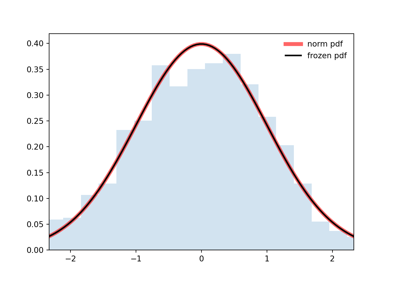
```{python}
#| label: A03-2
import numpy as np
from scipy.stats import norm
import matplotlib.pyplot as plt
fig, ax = plt.subplots(1, 1)

n, p = 5, 0.4
mean, var, skew, kurt = norm.stats(moments='mvsk')
print(f'{mean=:1.2f}, {var=:1.2f}, {skew=:1.2f}, {kurt=:1.2f}')
x = np.linspace(norm.ppf(0.01),
                norm.ppf(0.99), 100)
ax.plot(x, norm.pdf(x),
       'r-', lw=5, alpha=0.6, label='norm pdf')

rv = norm()
ax.plot(x, rv.pdf(x), 'k-', lw=2, label='frozen pdf')
r = norm.rvs(size=1000)

ax.hist(r, density=True, bins='auto', histtype='stepfilled', alpha=0.2)
ax.set_xlim([x[0], x[-1]])
ax.legend(loc='best', frameon=False)
plt.show()
```
## The t-Distribution {#sec-the-t-distribution}
\index{distribution!t}
If we have normal data, we can use (@eq-normal-sum) to help us estimate the mean $\mu$. Reversing the transformation from the previous section, we get:
$$
\frac {\hat X - \mu}{\sigma / \sqrt(n)} \sim N(0, 1)
$$ {#eq-t-transform}
However, we may not know the value of $\sigma$. If we estimate it from data, we can replace it with $S = \sqrt{\sum_i \frac{(X_i-\hat X)^2}{n-1}}$, the sample standard deviation. This causes the expression (@eq-t-transform) to no longer be distributed as a Standard Normal; but as a standard *t-distribution* with $ν = n − 1$ `degrees of freedom`
$$
X \sim t[\nu]
$$ {#eq-t-rv}
$$f(t\mid\nu) = \frac{\Gamma(\frac{\nu+1}{2})}{\Gamma(\frac{\nu}{2})\sqrt{\nu\pi}}\left (1 + \frac{t^2}{\nu}\right)^{-(\frac{\nu+1}{2})}\mathbb{I}_{t\in\mathbb{R}} \qquad \text{(PDF)}
$$ {#eq-t-pdf-gamma}
$$
\text{where }\Gamma(w)=\int_{0}^{\infty}t^{w-1}e^{-t}\mathrm{d}t \text{ is the gamma function}
$$
$$f(t\mid\nu)={\frac {1}{{\sqrt {\nu }}\,\mathrm {B} ({\frac {1}{2}},{\frac {\nu }{2}})}}\left(1+{\frac {t^{2}}{\nu }}\right)^{-(\nu +1)/2}\mathbb{I}_{t\in\mathbb{R}} \qquad \text{(PDF)}
$$ {#eq-t-pdf-beta}
$$
\text{where } B(u,v)=\int_{0}^{1}t^{u-1}(1-t)^{v-1}\mathrm{d}t \text{ is the beta function}
$$
$$\begin{aligned}
&& F(t)&=\int _{-\infty }^{t}f(u)\,du=1-{\tfrac {1}{2}}I_{x(t)}\left({\tfrac {\nu }{2}},{\tfrac {1}{2}}\right) &&\text{(CDF)} \\
\text{where } && I_{x(t)}&= \frac{B(x; u, v)}{B(u,v)} &&\text{is the regularized Beta function} \\
\text{where } && B(w; u,v)&=\int_{0}^{w}t^{u-1}(1-t)^{v-1}\mathrm{d}t && \text{ is the incomplete Beta function } \\
\text {and } && B(u,v)&=\int_{0}^{1}t^{u-1}(1-t)^{v-1}\mathrm{d}t && \text{ is the (complete) beta function}
\end{aligned}
$$ {#eq-t-cdf}
$$\int _{-\infty }^{t}f(u)\,du={\tfrac {1}{2}}+t{\frac {\Gamma \left({\tfrac {1}{2}}(\nu +1)\right)}{{\sqrt {\pi \nu }}\,\Gamma \left({\tfrac {\nu }{2}}\right)}}\,{}_{2}F_{1}\left({\tfrac {1}{2}},{\tfrac {1}{2}}(\nu +1);{\tfrac {3}{2}};-{\tfrac {t^{2}}{\nu }}\right)
$$
$$
\mathcal{L}(\mu, \sigma, \nu) = \prod_{i=1}^n \frac{\Gamma(\frac{\nu+1}{2})}{\sqrt{\nu\pi}\Gamma(\frac{\nu}{2})} \left(1+\frac{(x_i-\mu)^2}{\sigma^2\nu}\right)^{-\frac{\nu+1}{2}}
$$ {#eq-t-likelihood}
$$
\begin{aligned}
\ell(\mu, \sigma, \nu) &= \log \mathcal{L}(\mu, \sigma, \nu) \\
&= \sum_{i=1}^n \left[\log\Gamma\left(\frac{\nu+1}{2}\right) - \log\sqrt{\nu\pi} - \log\Gamma\left(\frac{\nu}{2}\right) - \frac{\nu+1}{2}\log\left(1+\frac{(x_i-\mu)^2}{\sigma^2\nu}\right)\right] \\
&= n\log\Gamma\left(\frac{\nu+1}{2}\right) - n\log\sqrt{\nu\pi} - n\log\Gamma\left(\frac{\nu}{2}\right) - \frac{\nu+1}{2}\sum_{i=1}^n\log\left(1+\frac{(x_i-\mu)^2}{\sigma^2\nu}\right).
\end{aligned}
$$ {#eq-t-log-likelihood}
$$
\mathbb{E}[Y] = 0 \qquad \text{ if } \nu > 1
$$ {#eq-t-expectation-xyz}
$$
\mathbb{V}ar[Y] = \frac{\nu}{\nu - 2} \qquad \text{ if } \nu > 2
$$ {#eq-t-variance}
## Location Scale Parametrization t-distribution
$$
X=\mu+\sigma T
$$
The resulting distribution is also called the non-standardized Student's t-distribution.
this is another parameterization of the student-t with:
- location $\mu \in \mathbb{R}^+$
- scale $\sigma \in \mathbb{R}^+$
- degrees of freedom $\nu \in \mathbb{R}^+$
$$
f(x \mid \mu, \sigma, \nu) = \frac{\left(\frac{\nu }{\nu +\frac{(x-\mu )^2}{\sigma ^2}}\right)^{\frac{\nu+1}{2}}}{\sqrt{\nu } \sigma B\left(\frac{\nu }{2},\frac{1}{2} \right)}
$$ {#eq-t-alt-pdf}
$$
\text{where } B(u,v)=\int_{0}^{1}t^{u-1}(1-t)^{v-1}\mathrm{d}t \text{ is the beta function}
$$
$$
F(\mu, \sigma, \nu) =
\begin{cases}
\frac{1}{2} I_{\frac{\nu \sigma ^2}{(x-\mu )^2+\nu \sigma ^2}}\left(\frac{\nu }{2},\frac{1}{2}\right), & x\leq \mu \\
\frac{1}{2} \left(I_{\frac{(x-\mu )^2}{(x-\mu )^2+\nu \sigma ^2}}\left(\frac{1}{2},\frac{\nu }{2}\right)+1\right), & \text{Otherwise}
\end{cases}
$$ {#eq-t-alt-cdf}
where $I_w(u,v)$ is the regularized incomplete beta function:
$$
I_w(u,v) = \frac{B(w; u, v)}{B(u,v)}
$$
where B(w; u,v) is the *incomplete beta function*:
$$
B(w; u,v) =\int_{0}^{w}t^{u-1}(1-t)^{v-1}\mathrm{d}t
$$
And $B(u,v)$ is the (complete) beta function
$$
\mathbb{E}[X] =
\begin{cases}
\mu, & \text{if }\nu > 1 \\
\text{undefined} & \text{ otherwise}
\end{cases}
$$ {#eq-t-alt-expectation}
$$
\mathbb{V}ar[X] = \frac{\nu \sigma^2}{\nu-2}
$$ {#eq-t-alt-variance}
The *t distribution* is symmetric and resembles the Normal Distribution but with thicker tails. As the degrees of freedom increase, the t distribution looks more and more like the standard normal distribution.
{#fig-bio-student .column-margin width="53mm"}
::: {.callout-tip .column-page-inset }
### Historical Note on The William Sealy Gosset A.K.A Student
\index{Gosset, William Sealy}
The student-t distribution is due to Gosset, William Sealy (1876-1937) who was an English statistician, chemist and brewer who served as Head Brewer of Guinness and Head Experimental Brewer of Guinness and was a pioneer of modern statistics. He is known for his pioneering work on small **sample experimental designs**. Gosset published under the pseudonym "Student" and developed most famously Student's t-distribution -- originally called Student's "z" -- and "Student's test of statistical significance".
He was told to use a Pseudonym and choose 'Student' after a predecessor at Guinness published a paper that leaked trade secrets. Gosset was a friend of both Karl Pearson and Ronald Fisher. Fisher suggested a correction to the student-t using the degrees of freedom rather than the sample size. Fisher is also credited with helping to publicize its use.
for a full biography see [@pearson1990student]
:::
## The Exponential Distribution {#sec-the-exponential-distribution}
\index{distribution!exponential}
### Story
The *Exponential distribution* models the waiting time between events for events with a rate lambda. Those events, typically, come from a `Poisson` process
The *exponential distribution* is often used to model the waiting time between random events. Indeed, if the waiting times between successive events are independent then they form an $Exp(λ)$ distribution. Then for any fixed time window of length t, the number of events occurring in that window will follow a *Poisson distribution* with mean $tλ$.
$$
X \sim Exp[\lambda]
$$ {#eq-exponential-rv}
### PDF
$$
f(x \mid \lambda) = \frac{1}{\lambda} e^{- \frac{x}{\lambda}}(x)\mathbb{I}_{\lambda\in\mathbb{R}^+ } \mathbb{I}_{x\in\mathbb{R}^+_0 } \quad \text{(PDF)}
$$ {#eq-exponential-pdf}
### CDF
$$
F(x \mid \lambda) = 1 - e^{-\lambda x} \qquad \text{(CDF)}
$$
$$
\mathcal{L}(\lambda) = \prod_{i=1}^n \lambda e^{-\lambda x_i}
$$ {#eq-exponential-likelihood}
$$
\begin{aligned} \ell(\lambda) &= \log \mathcal{L}(\lambda) \\
&= \sum_{i=1}^n \log(\lambda) - \lambda x_i \\
&= n\log(\lambda) - \lambda\sum_{i=1}^n x_i \end{aligned}
$$ {#eq-exponential-log-likelihood}
### Moments
$$
\mathbb{E}(x)= \lambda
$$ {#eq-exponential-expectation}
$$
\mathbb{V}ar[X]= \lambda^2
$$ {#eq-exponential-variance}
$$
\mathbb{M}_X(t)= \frac{1}{1-\lambda t} \qquad t < \frac{1}{\gamma}
$$ {#eq-exponential-mgf}
### Special cases:
\index{distribution!Weibull}
\index{distribution!Rayleigh}
\index{distribution!Gumbel}
- **Weibull** $Y = X^{\frac{1}{\gamma}}$
- **Rayleigh** $Y = \sqrt{\frac{2X}{\lambda}}$
- **Gumbel** $Y=\alpha - \gamma \log(\frac{X}{\lambda})$
### Properties:
- memoryless
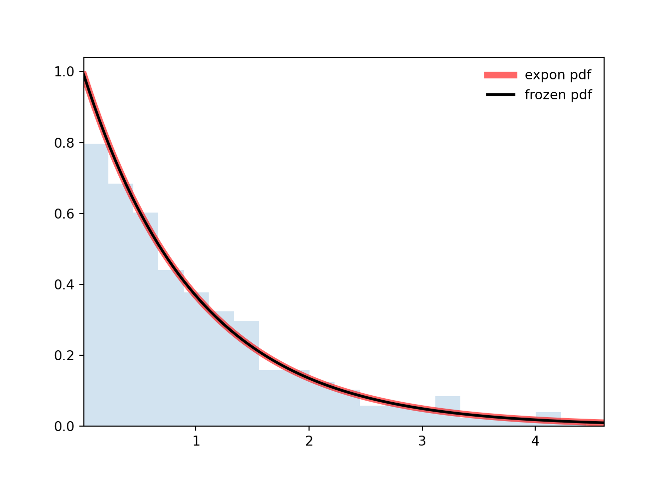
```{python}
#| label: A03-3
import numpy as np
from scipy.stats import expon
import matplotlib.pyplot as plt
fig, ax = plt.subplots(1, 1)

n, p = 5, 0.4
mean, var, skew, kurt = expon.stats(moments='mvsk')
print(f'{mean=:1.2f}, {var=:1.2f}, {skew=:1.2f}, {kurt=:1.2f}')
x = np.linspace(expon.ppf(0.01), expon.ppf(0.99), 100)
ax.plot(x, expon.pdf(x), 'r-', lw=5, alpha=0.6, label='expon pdf')

rv = expon()
ax.plot(x, rv.pdf(x), 'k-', lw=2, label='frozen pdf')

r = expon.rvs(size=1000)

ax.hist(r, density=True, bins='auto', histtype='stepfilled', alpha=0.2)
ax.set_xlim([x[0], x[-1]])
ax.legend(loc='best', frameon=False)
plt.show()
```
## LogNormal Distribution {#sec-lognormal-distribution}
The long normal arises when the a log transform is applied to the normal distribution.
\index{distribution!LogNormal}
$$
\text{LogNormal}(y\mid\mu,\sigma) = \frac{1}{\sqrt{2 \pi} \ \sigma} \, \frac{1}{y} \ \exp \! \left( - \, \frac{1}{2} \, \left( \frac{\log y - \mu}{\sigma} \right)^2 \right) \ \mathbb{I}_{\mu \in \mathbb{R}}\mathbb{I}_{\sigma \in \mathbb{R}^+}\mathbb{I}_{y \in \mathbb{R}^+} \qquad \text (PDF)
$$ {#eq-LogNormal-pdf}
## Pareto Distribution {#sec-pareto-distribution}
\index{distribution!Pareto}
$$
\text{Pareto}(y|y_{\text{min}},\alpha) = \frac{\displaystyle
\alpha\,y_{\text{min}}^\alpha}{\displaystyle y^{\alpha+1}} \mathbb{I}_{\alpha \in \mathbb{R}^+}\mathbb{I}_{y_{min} \in \mathbb{R}^+}\mathbb{I}_{y\ge y_{min} \in \mathbb{R}^+}
\qquad \text (PDF)
$$ {#eq-Pareto-pdf}
$$
\mathrm{Pareto\_Type\_2}(y|\mu,\lambda,\alpha) = \
\frac{\alpha}{\lambda} \, \left( 1+\frac{y-\mu}{\lambda}
\right)^{-(\alpha+1)} \! \mathbb{I}_{\mu \in \mathbb{R}}\mathbb{I}_{\lambda \in \mathbb{R}^+}\mathbb{I}_{\alpha \in \mathbb{R}^+}\mathbb{I}_{y\ge \mu \in \mathbb{R}}
\qquad \text (PDF)
$$ {#eq-Pareto2-pdf}
$$
\mathbb{E}[X]=\displaystyle{\frac{\alpha y_\mathrm{min}}{\alpha - 1}}\mathbb{I}_{\alpha>1} \qquad \text (expectation)
$$ {#eq-Pareto-expectation}
$$
\mathbb{V}ar[X]=\displaystyle{\frac{\alpha y_\mathrm{min}^2}{(\alpha - 1)^2(\alpha - 2)}}\mathbb{I}_{\alpha>2} \qquad \text (variance)
$$ {#eq-Pareto-variance}
## Weibull Distribution {#sec-weibull-distribution}
\index{distribution!Weibull}
### PDF
$$
\text{Weibull}(y|\alpha,\sigma) =
\frac{\alpha}{\sigma} \, \left( \frac{y}{\sigma} \right)^{\alpha - 1} \, e^{ - \left( \frac{y}{\sigma} \right)^{\alpha}} \mathbb{I}_{\alpha \in \mathbb{R}^+}\mathbb{I}_{\sigma \in \mathbb{R}^+}\mathbb{I}_{y \in \mathbb{R}^+} \qquad \text (PDF)
$$
## Chi Squared Distribution {#sec-chi-squared-distribution}
\index{distribution!Chi Squared}
The chi squared distribution is a special case of the gamma. It is widely used in hypothesis testing and the construction of confidence intervals. It is parameterized using parameter $\nu$ for the degrees of predom
### PDF:
$$
\text{ChiSquare}(y\mid\nu) = \frac{2^{-\nu/2}} {\Gamma(\nu / 2)} \,
y^{\nu/2 - 1} \, \exp \! \left( -\, \frac{1}{2} \, y \right) \mathbb{I}_{\nu \in \mathbb{R}^+}\mathbb{I}_{y \in \mathbb{R}} \qquad \text (PDF)
$$ {#eq-ChiSquare-pdf}
### CDF:
$$
{\frac {1}{\Gamma (\nu/2)}}\;\gamma \left({\frac {\nu}{2}},\,{\frac {x}{2}}\right) \qquad \text (CDF)
$$ {#eq-ChiSquare-cdf}
### MOMENTS
$$
\mathbb{E}[X]=\nu
$$ {#eq-ChiSquare-expectation}
$$
\mathbb{V}ar[X] = 2\nu
$$ {#eq-ChiSquare-variance}
## Logistic Distribution {#sec-logistic-distribution}
\index{distribution!logistic}
$$\text{Logistic}(y|\mu,\sigma) = \frac{1}{\sigma} \
\exp\!\left( - \, \frac{y - \mu}{\sigma} \right) \ \left(1 + \exp
\!\left( - \, \frac{y - \mu}{\sigma} \right) \right)^{\!-2} \mathbb{I}_{\mu \in \mathbb{R}}\mathbb{I}_{\sigma \in \mathbb{R}^+}\mathbb{I}_{y \in \mathbb{R}} \qquad \text (PDF)
$$ {#eq-Logistic-pdf}
## F Distribution {#sec-f-distribution}
\index{distribution!F}
\index{F-ratio}
[F Distribution]{.column-margin} [F-ratio]{.column-margin} The F-distribution or F-ratio, arises frequently as the null distribution of a test statistic, in the analysis of variance (ANOVA) and other F-tests.
### PDF
$$
\frac {\sqrt {\frac {(d_{1}x)^{d_{1}}d_{2}^{d_{2}}}{(d_{1}x+d_{2})^{d_{1}+d_{2}}}}}{x\,\mathrm {B} \!\left({\frac {d_{1}}{2}},{\frac {d_{2}}{2}}\right)}
$$ {#eq-f-pdf}
### CDF
$$
\mathbb{I}_{\frac {d_{1}x}{d_{1}x+d_{2}}}\left({\tfrac {d_{1}}{2}},{\tfrac {d_{2}}{2}}\right)
$$ {#eq-f-cdf}
### Moments
$$
\mathbb{E}[X]=\frac {d_{2}}{d_{2}-2}
$$ {#eq-f-mean}
$$
\mathbb{V}ar[X] = {\frac {2\,d_{2}^{2}\,(d_{1}+d_{2}-2)}{d_{1}(d_{2}-2)^{2}(d_{2}-4)}}
$$ {#eq-f-variance}