oring=read.table("data/challanger.txt", header=T)
# Note that attaching this masks T which is originally TRUE
attach(oring)Recall that linear regression is a model for predicting a response or dependent variable (Y, also called an output) from one or more covariates or independent variables (X, also called explanatory variables, inputs, or features). For a given value of a single x, the expected value of y is
\mathbb{E}[y] = \beta_0 + \beta_1x
or we could say that
Y \sim \mathcal{N}(\beta_0 + \beta_1x, \sigma^2)
For data (x_1, y_1), \dots , (x_n, y_n), the fitted values for the coefficients, \hat{\beta_0} and \hat{\beta_1} are those that minimize the sum of squared errors \sum_{i = 1}^n{(y_i - \hat{y_i})^2}, where the predicted values for the response are \hat{y} = \hat{\beta_0} + \hat{\beta_1}x. We can get these values from R. These fitted coefficients give the least-squares line for the data.
This model extends to multiple covariates, with one \beta_j for each k covariates
\mathbb{E}[y_i] = \beta_0 + \beta_1x_{i1} + \dots + \beta_kx_{ik}
Optionally, we can represent the multivariate case using vector-matrix notation.
27.1 Conjugate Modeling
In the Bayesian framework, we treat the \beta parameters as unknown, put a prior on them, and then find the posterior. We might treat \sigma^2 as fixed and known, or we might treat it as an unknown and also put a prior on it. Because the underlying assumption of a regression model is that the errors are independent and identically normally distributed with mean 0 and variance \sigma^2, this defines a normal likelihood.
27.1.1 \sigma^2 known
Sometimes we may know the value of the error variance \sigma^2 . This simplifies calculations. The conjugate prior for the \beta is a normal prior. In practice, people typically use a non-informative prior, i.e., the limit as the variance of the normal prior goes to infinity, which has the same mean as the standard least-squares estimates. If we are only estimating \beta and treating \sigma^2 as known, then the posterior for \beta is a (multivariate) normal distribution. If we just have a single covariate, then the posterior for the slope is:
\beta_1 \mid y \sim N\left(\frac{\sum_{i = 1}^n{(x_i-\bar{x})(y_i - \bar{y})}}{\sum_{i=1}^n{(x_i-\bar{x})^2}}, \frac{\sigma^2}{\sum_{i=1}^n{(x_i - \bar{x})^2}}\right)
If we have multiple covariates, then using a matrix-vector notation, the posterior for the vector of coefficients is \beta \mid y \sim N((X^tX)^{-1}X^ty, (X^tX)^{-1}\sigma^2)
where X denotes the design matrix and X^t is the transpose of X. The intercept is typically included in X as a column of 1’s. Using an improper prior requires us to have at least as many data points as we have parameters to ensure that the posterior is proper.
27.1.2 \sigma^2 Unknown
If we treat both \beta and \sigma^2 as unknown, the standard prior is the non-informative Jeffreys prior, f(\beta, \sigma^2) \propto \frac{1}{\sigma^2} . Again, the posterior mean for \beta will be the same as the standard least-squares estimates. The posterior for \beta conditional on \sigma^2 is the same normal distributions as when \sigma^2 is known, but the marginal posterior distribution for \beta, with \sigma^2 integrated out is a t distribution, analogous to the t tests for significance in standard linear regression. The posterior t distribution has mean (X^tX)^{-1}X^ty and scale matrix (related to the variance matrix) s^2(X^tX)^{-1} , where s^2 = \sum_{i = 1}^n{(y_i - \hat{y_i})^2/(n - k - 1)} . The posterior distribution for \sigma^2 is an inverse gamma distribution
\sigma^2 \mid y \sim \Gamma^{-1}(\frac{n - k - 1}{2}, \frac{n - k - 1}{2}s^2)
In the simple linear regression case (single variable), the marginal posterior for \beta is a t distribution with mean \frac{\sum_{i = 1}^n{(x_i-\bar{x})(y_i - \bar{y})}}{\sum_{i=1}^n{(x_i-\bar{x})^2}} and scale \frac{s^2}{\sum_{i=1}^n{(x_i - \bar{x})^2}} . If we are trying to predict a new observation at a specified input x^* , that predicted value has a marginal posterior predictive distribution that is a t distribution, with mean \hat{y} = \hat{\beta_0} + \hat{\beta_1}x^* and scale se_r\sqrt{1 + \frac{1}{n} + \frac{(x^* - \bar{x})^2}{(n - 1)s_x^2}} . se_r is the residual standard error of the regression, which can be found easily in R. s_x^2 is the sample variance of x. Recall that the predictive distribution for a new observation has more variability than the posterior distribution for \hat{y}, because individual observations are more variable than the mean.
27.2 Linear Regression
27.2.1 Single Variable Regression
We’ll be looking at the Challenger dataset. It contains 23 past launches where it has the temperature at the day of launch and the O-ring damage index
Read in the data https://pdixon.stat.iastate.edu/stat511/datasets/challenger2.txt
head(oring) t i
1 53 11
2 57 4
3 58 4
4 63 2
5 66 0
6 67 0Now we’ll see the plot
plot(t,i)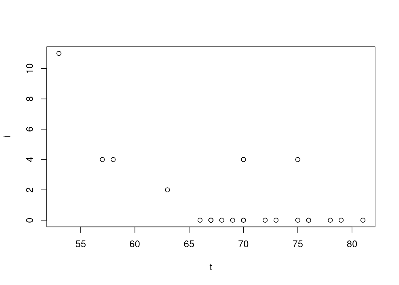
Fit a linear model
oring.lm = lm(i ~ t)
summary(oring.lm)
Call:
lm(formula = i ~ t)

Residuals:
    Min      1Q  Median      3Q     Max
-2.3025 -1.4507 -0.4928  0.7397  5.5337

Coefficients:
            Estimate Std. Error t value Pr(>|t|)
(Intercept) 18.36508    4.43859   4.138 0.000468 ***
t           -0.24337    0.06349  -3.833 0.000968 ***
---
Signif. codes:  0 '***' 0.001 '**' 0.01 '*' 0.05 '.' 0.1 ' ' 1

Residual standard error: 2.102 on 21 degrees of freedom
Multiple R-squared:  0.4116,    Adjusted R-squared:  0.3836
F-statistic: 14.69 on 1 and 21 DF,  p-value: 0.0009677
Add the fitted line into the scatter plot
plot(t,i)
lines(t,fitted(oring.lm)) 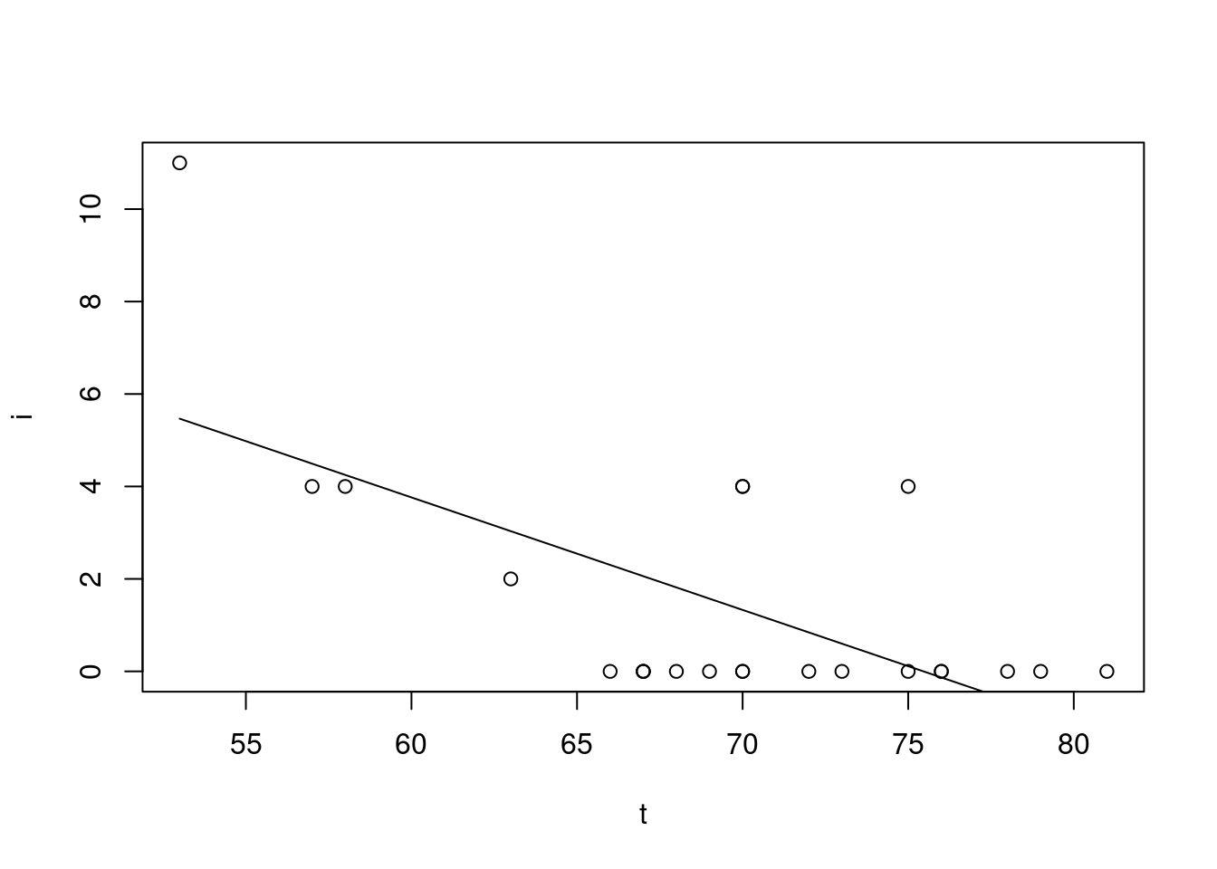
Create a 95% posterior interval for the slope
-0.24337 - 0.06349*qt(.975,21)[1] -0.3754047-0.24337 + 0.06349*qt(.975,21)[1] -0.1113353Note: These are the same as the frequentist confidence intervals
If the challenger launch was at 31 degrees Fahrenheit, how much O-Ring damage would we predict?
coef(oring.lm)[1] + coef(oring.lm)[2]*31 (Intercept)
10.82052 # [1] 10.82052 Let’s make our posterior prediction interval
predict(oring.lm,data.frame(t=31),interval="predict") fit lwr upr
1 10.82052 4.048269 17.59276We can calculate the lower bound through the following formula
10.82052-2.102*qt(.975,21)*sqrt(1+1/23+((31-mean(T))^2/22/var(t)))[1] 4.850937What’s the posterior probability that the damage index is greater than zero?
1-pt((0-10.82052)/(2.102*sqrt(1+1/23+((31-mean(T))^2/22/var(T)))),21)[1] NA27.2.2 Multivariate Regression
We’re looking at Galton’s seminal data predicting the height of children from the height of the parents.
  Family Father Mother Gender Height Kids
1      1   78.5   67.0      M   73.2    4
2      1   78.5   67.0      F   69.2    4
3      1   78.5   67.0      F   69.0    4
4      1   78.5   67.0      F   69.0    4
5      2   75.5   66.5      M   73.5    4
6      2   75.5   66.5      M   72.5    4
7      2   75.5   66.5      F   65.5    4
8      2   75.5   66.5      F   65.5    4
What are the columns in the dataset?
names(heights)[1] "Family" "Father" "Mother" "Gender" "Height" "Kids" # [1] "Family" "Father" "Mother" "Gender" "Height" "Kids" explanation of the columns:
- Family: the family the child is from
- Father: height of the father
- Mother: height of the mother
- Kids: count of children in the family
- Gender: the gender of the child
- Height: the height the child
The Height is out target variables.
Let’s look at the relationship between the different variables
pairs(heights)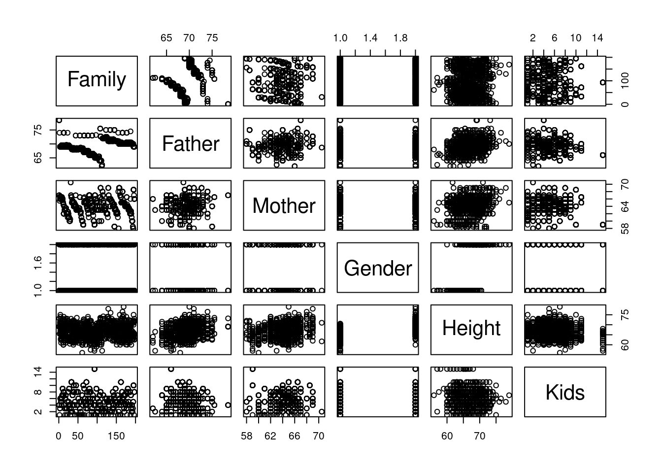
Pair plots are a great tool for doing EDA in R. You need to get used read them.
We care primarily about the Height so we can should first consider the row of the height. The other rows can inform us if there is a relation between other variables.
- the Father and Mother are correlated with height.
- Gender male children are generally taller.
- Kids and Family don’t seem to have a clear pattern.
First let’s start by creating a linear model taking all of the columns into account
summary(lm(Height~Father+Mother+Gender+Kids))
Call:
lm(formula = Height ~ Father + Mother + Gender + Kids)

Residuals:
    Min      1Q  Median      3Q     Max
-9.4748 -1.4500  0.0889  1.4716  9.1656

Coefficients:
            Estimate Std. Error t value Pr(>|t|)
(Intercept) 16.18771    2.79387   5.794 9.52e-09 ***
Father       0.39831    0.02957  13.472  < 2e-16 ***
Mother       0.32096    0.03126  10.269  < 2e-16 ***
GenderM      5.20995    0.14422  36.125  < 2e-16 ***
Kids        -0.04382    0.02718  -1.612    0.107
---
Signif. codes:  0 '***' 0.001 '**' 0.01 '*' 0.05 '.' 0.1 ' ' 1

Residual standard error: 2.152 on 893 degrees of freedom
Multiple R-squared:  0.6407,    Adjusted R-squared:  0.6391
F-statistic: 398.1 on 4 and 893 DF,  p-value: < 2.2e-16
As you can see here, the Kids column is not statistically significant. Let’s look at a model with it removed.
heights.lm=lm(Height~Father+Mother+Gender)
summary(heights.lm)
Call:
lm(formula = Height ~ Father + Mother + Gender)

Residuals:
   Min     1Q Median     3Q    Max
-9.523 -1.440  0.117  1.473  9.114

Coefficients:
            Estimate Std. Error t value Pr(>|t|)
(Intercept) 15.34476    2.74696   5.586 3.08e-08 ***
Father       0.40598    0.02921  13.900  < 2e-16 ***
Mother       0.32150    0.03128  10.277  < 2e-16 ***
GenderM      5.22595    0.14401  36.289  < 2e-16 ***
---
Signif. codes:  0 '***' 0.001 '**' 0.01 '*' 0.05 '.' 0.1 ' ' 1

Residual standard error: 2.154 on 894 degrees of freedom
Multiple R-squared:  0.6397,    Adjusted R-squared:  0.6385
F-statistic:   529 on 3 and 894 DF,  p-value: < 2.2e-16
This model looks good. We can tell from the summary that:
- each extra inch of the father’s height contributes an extra 0.4 inches height of the child.
- each extra inch of the mother’s height contributes an extra 0.3 inches height of the child.
- male gender contributes 5.2 inches to the height of the child.
Let’s create a 95% posterior interval for the difference in height by gender
5.226 - 0.144 * qt(.975,894)[1] 4.9433835.226 + 0.144 * qt(.975,894)[1] 5.508617Let’s make a posterior prediction interval for a male and female with a father whose 68 inches and a mother whose 64 inches.
predict(heights.lm,data.frame(Father=68,Mother=64,Gender="M"), interval="predict") fit lwr upr
1 68.75291 64.51971 72.9861predict(heights.lm,data.frame(Father=68,Mother=64,Gender="F"), interval="predict") fit lwr upr
1 63.52695 59.29329 67.76062