x = seq(-3, 7, length=100)
y = 0.3*dnorm(x, 0, 1) + 0.7*dnorm(x, 4, 1)
par(mar=c(4,4,1,1)+0.1)
plot(x, y, type="l", ylab="Density", las=1, lwd=2)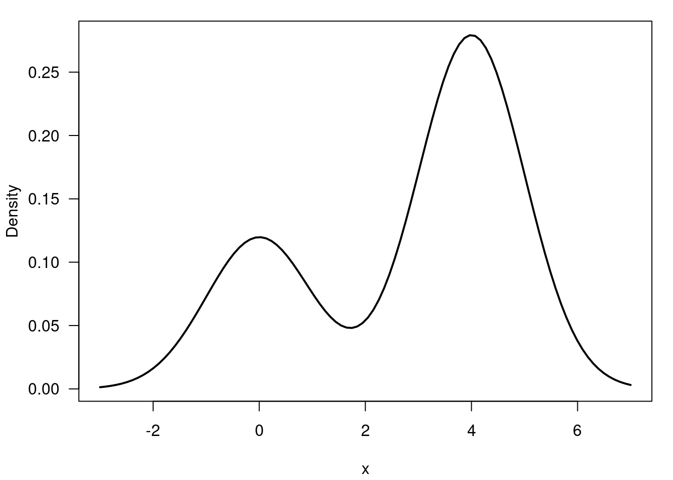
Mixture Models, Homework
Exercise 59.1 Which one of the following is not the density of a well defined mixture distribution with support on the positive integers:
POISSON(\lambda) = \frac{\lambda^x e^{-\lambda}}{x!}
\sum_{x=0}^{\infty} \frac{2^x e^{-1}}{x!} = e^{-1} \sum_{x=0}^{\infty} \frac{2^x}{x!} = e^{-1} e^{2} = e^{1}
the last one is not a well defined mixture distribution because exponent is has a lambda of 1 but should be 2 to be a poisson distribution.
Actually the answer is not 100% kosher as we have not demonstrated that it is not a well defined mixture distribution - we need to show it doesn’t sum to 1 or is not a valid distribution.
I have given this fact in the hint above.
Exercise 59.2 Consider a zero-inflated mixture that involves a point mass at 0 with weight 0.2, a Gamma distribution with mean 1, variance 2 and weight 0.5, and another Gamma distribution with mean 2, variance 4 and weight 0.3. What is the mean of this mixture?
E(X) = 0.2 \cdot 0 + 0.5 \cdot 1 + 0.3 \cdot 2 = 1.1
Exercise 59.3 Consider a zero-inflated mixture that involves a point mass at 0 with weight 0.2, a Gamma distribution with mean 1, variance 2 and weight 0.5, and another Gamma distribution with mean 2, variance 4 and weight 0.3. What is the variance of this mixture?
\begin{aligned} V[X] &= E[X^2] - E[X]^2 \\ &= (\sum_{i=1}^{n} w_i Var_{g_k}[X^2_i] + E_{g_k}[X]^2) - E[X]^2 \\ E[X^2] &= 0.2 \cdot 0^2 + 0.5 \cdot (1 + 1^2) + 0.3 \cdot (2 + 4) = 3.9 \\ V[X] &= 3.9 - 1.1^2 = 2.69 \end{aligned}
Exercise 59.4 True or False: A mixture of Gaussians of the form
f(x) = 0.3 \frac{1}{\sqrt{2 \pi}} e^{-\frac{x^2}{2}} + 0.7 \frac{1}{\sqrt{2 \pi}} e^{-\frac{(x-4)^2}{2}}
has a bimodal density.
According to the 68-95-99.7 rule, if two gaussian have means that are separated by distance greater than 1 sd apart, then the mixture should appear bimodal.
True. The two gaussians are separated by 4 standard deviations, so the mixture will be bimodal. We can verify this by plotting the density of the mixture.
x = seq(-3, 7, length=100)
y = 0.3*dnorm(x, 0, 1) + 0.7*dnorm(x, 4, 1)
par(mar=c(4,4,1,1)+0.1)
plot(x, y, type="l", ylab="Density", las=1, lwd=2)
Exercise 59.5 True or False: Consider a location mixture of normals f(x) = \sum_{k=1}^{K} \omega_k \frac{1}{\sqrt{2 \pi} \sigma} e^{-\frac{(x - \mu_k)^2}{2 \sigma^2}}
The following 3 constraints make all parameters fully identifiable:
True.
The first and second address the number of components, while the last deals with label switching.