---
title : 'Density Estimation - M4L5'
subtitle : 'Bayesian Statistics: Mixture Models - Applications'
categories:
- Bayesian Statistics
keywords:
- Mixture Models
- Kernel Density Estimation
- Mixture Density Estimation
- Clustering
- Classification
- notes
---
## Density Estimation using Mixture Models :movie_camera: {#sec-density-estimation-using-mixture-models}
{.column-margin width="53mm"}
### KDE
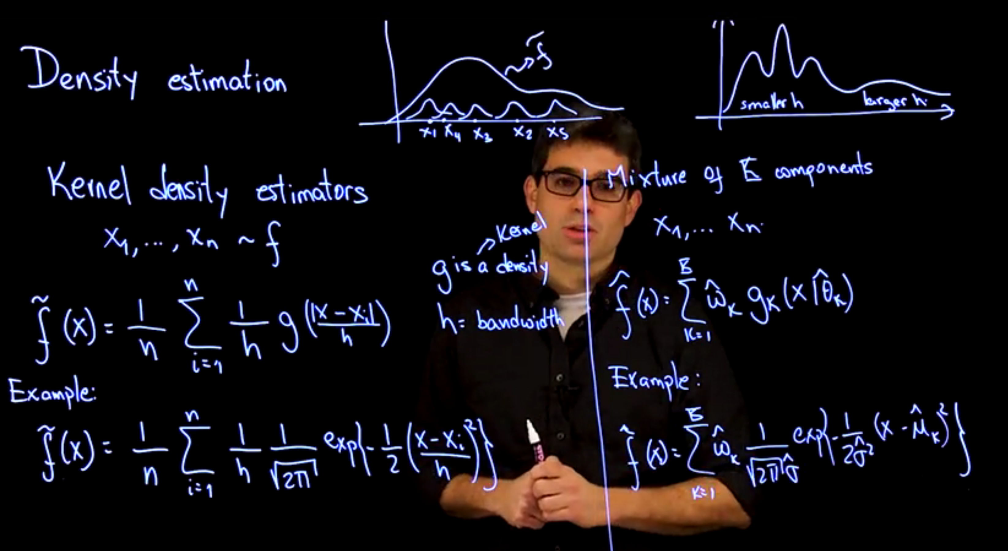
- the typical method for estimating the density of a random variable is to use a kernel density estimator (KDE)
- the KDE is a non-parametric method that estimates the density of a random variable by averaging the contributions of a set of kernel functions centered at each data point
$$
X_1, \ldots, X_n \sim f(x)
$$
$$
\tilde{f}(x) = \frac{1}{n} \sum_{i=1}^n \frac{1}{h} g \left (\frac{\|X - X_i\|}{h}\right )
$$ {#eq-kde-definition-for-density-estimation}
\index{bandwidth} \index{kernel function}
where $h$ is the bandwidth of the kernel and $g$ is a kernel function. The kernel function is a non-negative function that integrates to 1 and is symmetric around 0.
\index{Gaussian function}
For example, the Gaussian kernel is given by:
$$
g(x) = \frac{1}{\sqrt{2\pi}} e^{-\frac{x^2}{2}}
$$ {#eq-gaussian-kernel}
giving us:
$$
\tilde{f}(x) = \frac{1}{n} \sum_{i=1}^n \frac{1}{h} \frac{1}{\sqrt{2\pi}} e^{-\frac{|X - X_i|^2}{2h^2}}
$$ {#eq-kde}
### Mixture of K components
- a mixture of K components is a parametric method that estimates the density of a random variable by averaging the contributions of K kernel functions, each centered at a different location and with a different scale
- the mixture model is given by:
$$
X_1, \ldots, X_n \sim f(x) = \sum_{k=1}^K w_k g(x \mid \hat{\theta}_k)
$$ {#eq-mixture-density-estimation}
where $w_k$ is the weight of the $k$^-th^ component, $\hat{\theta}_k$ is the location and scale of the $k$^-th^ component, and $g(x \mid \hat{\theta}_k)$ is the kernel function centered at $\hat{\theta}_k$. The weights are non-negative and sum to 1.
Example: a location mixture of K Gaussian distributions is given by:
$$
X_1, \ldots, X_n \sim \hat{f}(x) = \sum_{k=1}^K \hat{w}_k \frac{1}{\sqrt{2\pi}\hat{\sigma}} \exp^{-\frac{(x - \hat{\mu}_k)^2}{2\hat{\sigma}^2}}
$$ {#eq-mixture-density-estimation-gaussian-location}
where $\hat{w}_k$ is the weight of the $k$^-th^ component, $\hat{\mu}_k$ is the mean of the $k$^-th^ component, and $\hat{\sigma}$ is the standard deviation of the $k$^-th^ component.
we can see the the two methods are quite similar, but the mixture model is more flexible and can capture more complex shapes in the data.
- The KDE is a special case of the mixture model where all the components have the same scale and location.
- KDE needs as many components as the number of data points, while the mixture model can have fewer components.
- KDE uses a fixed bandwidth,
- MDE can adaptively choose the bandwidth for each component. In fact we have a weight for each component and a scale parameter that controls the width of the kernel function.
- MDE tends to use less components and the weights tend to be 1/K
The above model can be improved by:
1. using a scale-location mixture model, where the scale and location of each component are estimated from the data.
### Density Estimation Example :movie_camera: {#sec-density-estimation-example}
\index{dataset!galaxies}
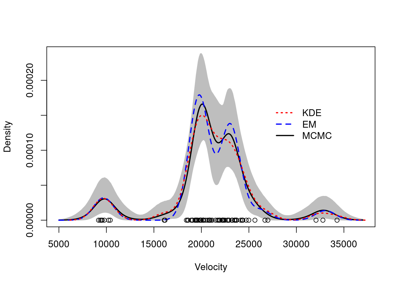
We use the galaxies dataset to illustrate the differences between the two methods.
The galaxies dataset contains the velocities of 82 galaxies in the Virgo cluster.
The data is available in the MASS package.
### Sample code for Density Estimation Problem
```{r}
#| label: "lbl-density-estimation-example"
## Using mixture models for density estimation in the galaxies dataset
## Compare kernel density estimation, and estimates from mixtures of KK=6
## components obtained using both frequentist and Bayesian procedures
rm(list=ls())

### Loading data and setting up global variables
library(MASS)
library(MCMCpack)
data(galaxies)
KK = 6          # Based on the description of the dataset
x  = galaxies
n  = length(x)
set.seed(781209)

### First, compute the "Maximum Likelihood" density estimate associated with a location mixture of 6 Gaussian distributions using the EM algorithm
## Initialize the parameters
w     = rep(1,KK)/KK
mu    = rnorm(KK, mean(x), sd(x))
sigma = sd(x)/KK

epsilon = 0.000001
s       = 0
sw      = FALSE
KL      = -Inf
KL.out  = NULL

while(!sw){
  ## E step
  v = array(0, dim=c(n,KK))
  for(k in 1:KK){
    v[,k] = log(w[k]) + dnorm(x, mu[k], sigma,log=TRUE)
  }
  for(i in 1:n){
    v[i,] = exp(v[i,] - max(v[i,]))/sum(exp(v[i,] - max(v[i,])))
  }

  ## M step
  # Weights
  w = apply(v,2,mean)
  mu = rep(0, KK)
  for(k in 1:KK){
    for(i in 1:n){
      mu[k]    = mu[k] + v[i,k]*x[i]
    }
    mu[k] = mu[k]/sum(v[,k])
  }
  # Standard deviations
  sigma = 0
  for(i in 1:n){
    for(k in 1:KK){
      sigma = sigma + v[i,k]*(x[i] - mu[k])^2
    }
  }
  sigma = sqrt(sigma/sum(v))

  ##Check convergence
  KLn = 0
  for(i in 1:n){
    for(k in 1:KK){
      KLn = KLn + v[i,k]*(log(w[k]) + dnorm(x[i], mu[k], sigma, log=TRUE))
    }
  }
  if(abs(KLn-KL)/abs(KLn)<epsilon){
    sw=TRUE
  }
  KL = KLn
  KL.out = c(KL.out, KL)
  s = s + 1
  print(paste(s, KLn))
}
xx  = seq(5000,37000,length=300)
nxx = length(xx)
density.EM = rep(0, nxx)
for(s in 1:nxx){
  for(k in 1:KK){
    density.EM[s] = density.EM[s] + w[k]*dnorm(xx[s], mu[k], sigma)
  }
}

### Get a "Bayesian" kernel density estimator based on the same location mixture of 6 normals
## Priors set up using an "empirical Bayes" approach
aa  = rep(1,KK)
eta = mean(x)
tau = sqrt(var(x))
dd  = 2
qq  = var(x)/KK

## Initialize the parameters
w     = rep(1,KK)/KK
mu    = rnorm(KK, mean(x), sd(x))
sigma = sd(x)/KK
cc    = sample(1:KK, n, replace=T, prob=w)

## Number of iterations of the sampler
rrr   = 12000
burn  = 2000

## Storing the samples
cc.out    = array(0, dim=c(rrr, n))
w.out     = array(0, dim=c(rrr, KK))
mu.out    = array(0, dim=c(rrr, KK))
sigma.out = rep(0, rrr)
logpost   = rep(0, rrr)


for(s in 1:rrr){
  # Sample the indicators
  for(i in 1:n){
    v = rep(0,KK)
    for(k in 1:KK){
      v[k] = log(w[k]) + dnorm(x[i], mu[k], sigma, log=TRUE)  #Compute the log of the weights
    }
    v = exp(v - max(v))/sum(exp(v - max(v)))
    cc[i] = sample(1:KK, 1, replace=TRUE, prob=v)
  }

  # Sample the weights
  w = as.vector(rdirichlet(1, aa + tabulate(cc, nbins=KK)))

  # Sample the means
  for(k in 1:KK){
    nk    = sum(cc==k)
    xsumk = sum(x[cc==k])
    tau2.hat = 1/(nk/sigma^2 + 1/tau^2)
    mu.hat  = tau2.hat*(xsumk/sigma^2 + eta/tau^2)
    mu[k]   = rnorm(1, mu.hat, sqrt(tau2.hat))
  }

  # Sample the variances
  dd.star = dd + n/2
  qq.star = qq + sum((x - mu[cc])^2)/2
  sigma = sqrt(1/rgamma(1, dd.star, qq.star))

  # Store samples
  cc.out[s,]   = cc
  w.out[s,]    = w
  mu.out[s,]   = mu
  sigma.out[s] = sigma
  for(i in 1:n){
    logpost[s] = logpost[s] + log(w[cc[i]]) + dnorm(x[i], mu[cc[i]], sigma, log=TRUE)
  }
  logpost[s] = logpost[s] + log(ddirichlet(w, aa))
  for(k in 1:KK){
    logpost[s] = logpost[s] + dnorm(mu[k], eta, tau, log=TRUE)
  }
  logpost[s] = logpost[s] + dgamma(1/sigma^2, dd, qq, log=TRUE) - 4*log(sigma)
  if(s/500==floor(s/500)){
    print(paste("s =",s))
  }
}
## Compute the samples of the density over a dense grid
density.mcmc = array(0, dim=c(rrr-burn,length(xx)))
for(s in 1:(rrr-burn)){
    for(k in 1:KK){
        density.mcmc[s,] = density.mcmc[s,] + w.out[s+burn,k]*dnorm(xx,mu.out[s+burn,k],sigma.out[s+burn])
    }
}
density.mcmc.m = apply(density.mcmc , 2, mean)

## Plot Bayesian estimate with pointwise credible bands along with kernel density estimate and frequentist point estimate
colscale = c("black", "blue", "red")
yy = density(x)
density.mcmc.lq = apply(density.mcmc, 2, quantile, 0.025)
density.mcmc.uq = apply(density.mcmc, 2, quantile, 0.975)
plot(xx, density.mcmc.m, type="n",ylim=c(0,max(density.mcmc.uq)),xlab="Velocity", ylab="Density")
polygon(c(xx,rev(xx)), c(density.mcmc.lq, rev(density.mcmc.uq)), col="grey", border="grey")
lines(xx, density.mcmc.m, col=colscale[1], lwd=2)
lines(xx, density.EM, col=colscale[2], lty=2, lwd=2)
lines(yy, col=colscale[3], lty=3, lwd=2)
points(x, rep(0,n))
legend(27000, 0.00017, c("KDE","EM","MCMC"), col=colscale[c(3,2,1)], lty=c(3,2,1), lwd=2, bty="n")
```