# Mixture of univariate Gaussians, bimodal
x = seq(-5, 12, length=100)
y = 0.6*dnorm(x, 0, 1) + 0.4*dnorm(x, 5, 2)


par(mar=c(4,4,1,1)+0.1)
plot(x, y, type="l", ylab="Density", las=1, lwd=2)
# set the title
title("Bimodal Mixture of Gaussians")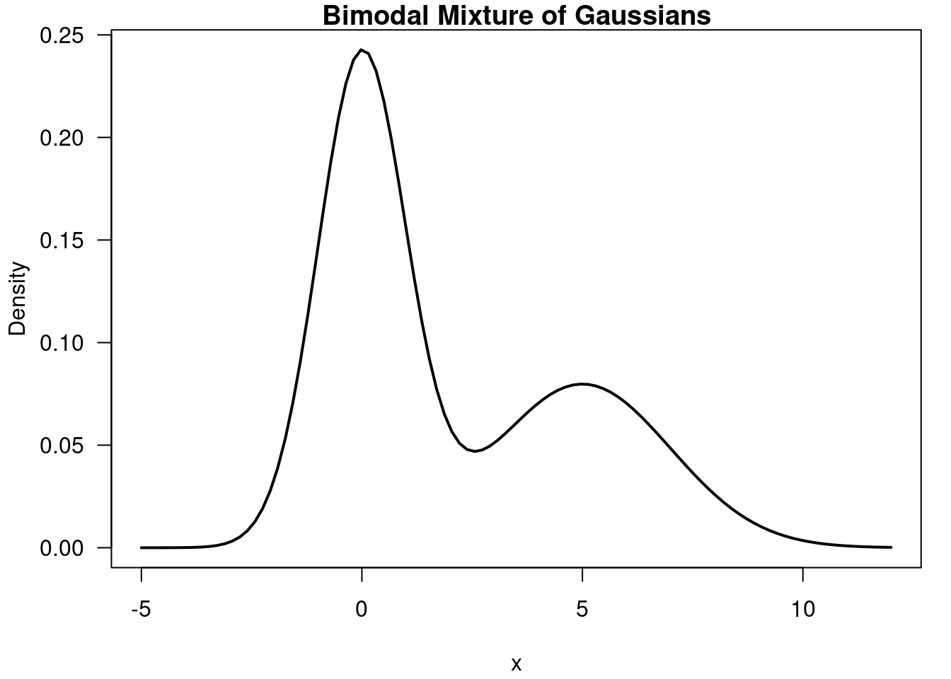
Mixture Models, notes
This module titled “Basic concepts on Mixture Models” defines mixture models, discusses their properties, and develops the likelihood function for a random sample from a mixture model that will be the basis for statistical learning.
The module begins with a welcome section and a video and a reading on installing as well as a 103 page long handout titled “introduction to R”. I skipped this obligatory section as I this has already been adequately covered in the notes for the previous courses.
This handout: Mixture model are the instructor notes for this course.
Mixture models provide a flexible approach to modeling data. We will soon learn how mixtures may be utilized for density estimation Section 73.1, clustering Section 74.1 and classification Section 75.1 problems:
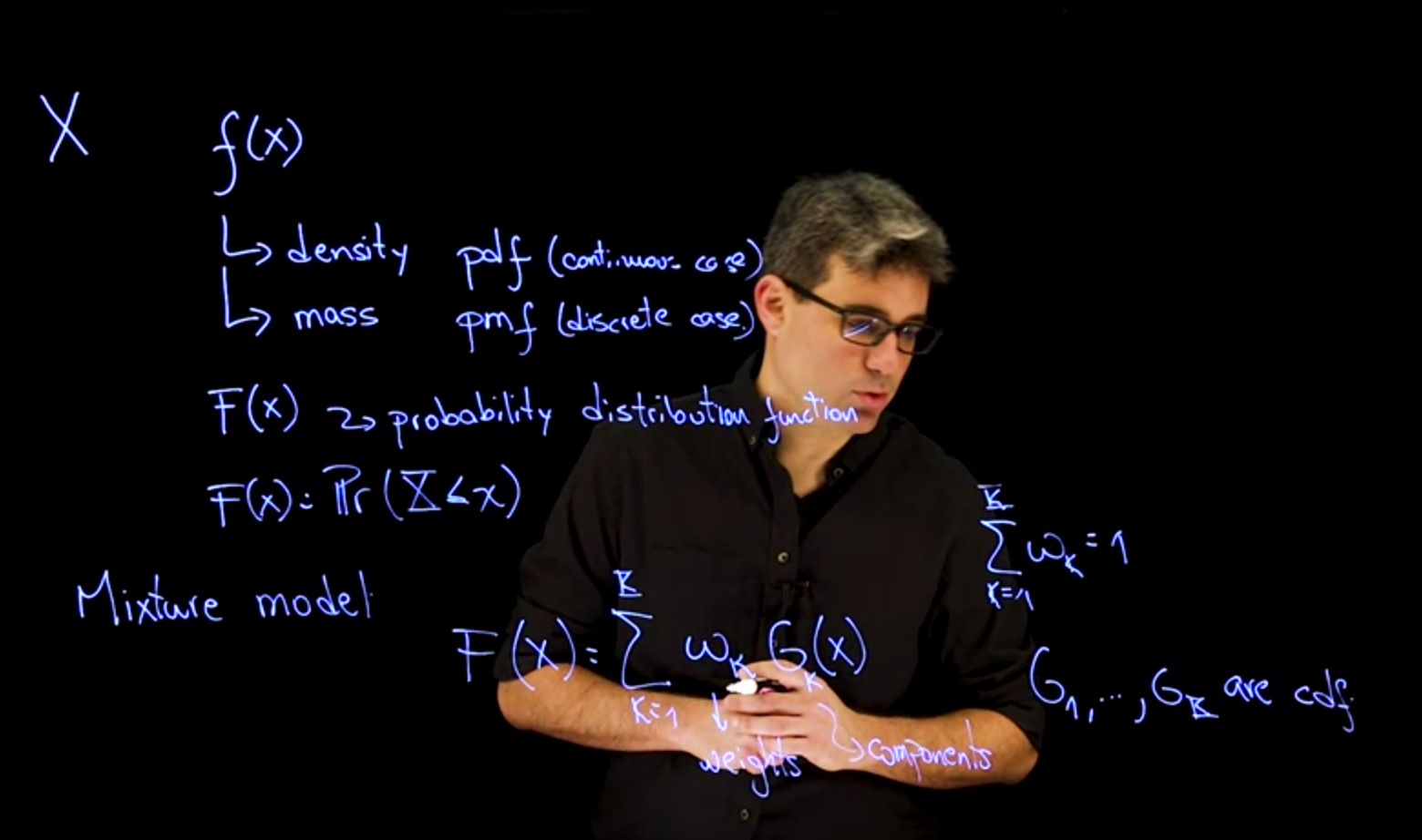
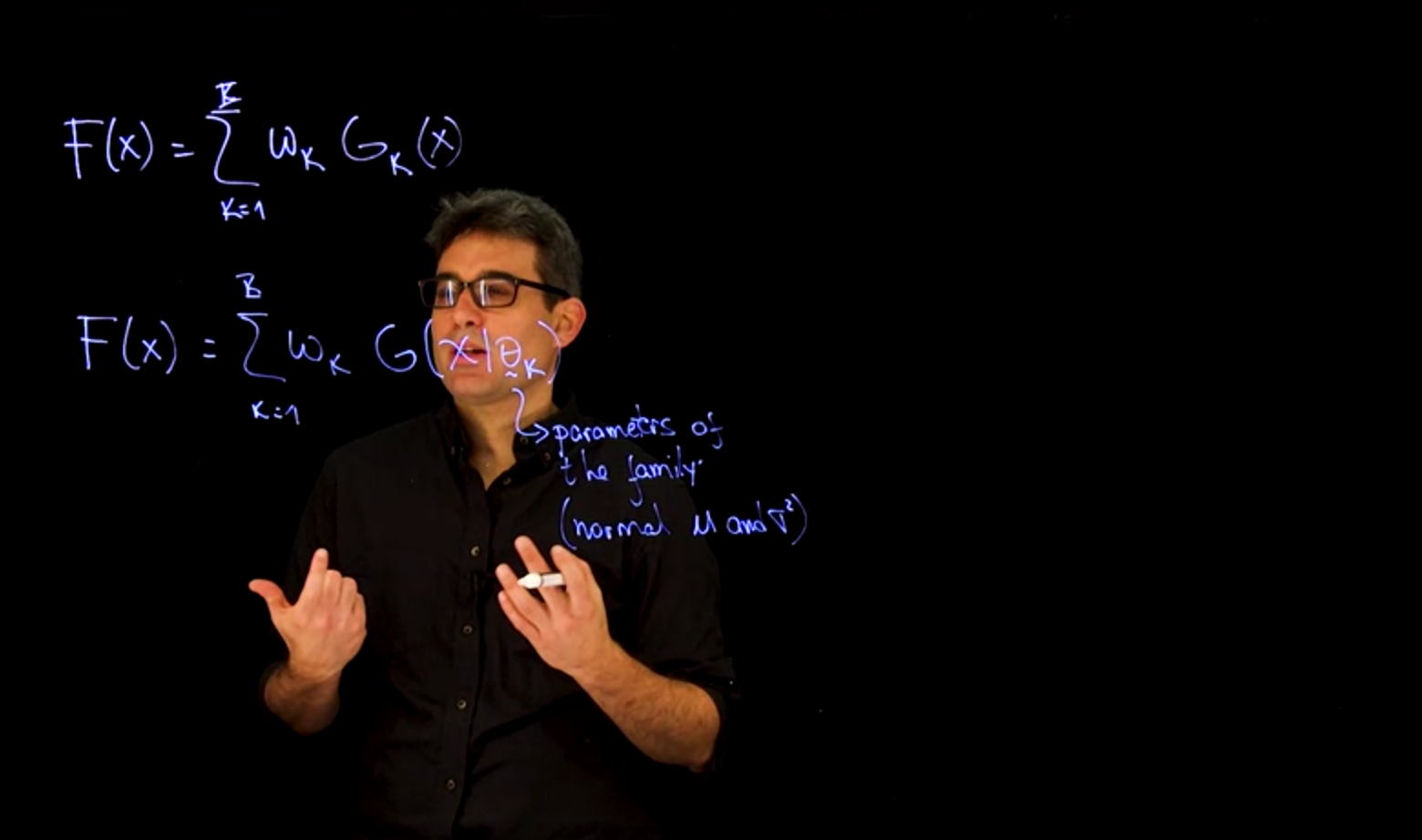
Definition 55.1 Let \omega_1 , \ldots , \omega_K be a collection of real numbers such that 0 \le \omega_k \le 1 and \sum^K_{k=1} \omega_k = 1, and G_1, \ldots, G_K be a collection of cumulative distribution functions. A random variable X with cumulative distribution function F(x) = Pr(X \le x) of the form:
F(x) =\sum^K_{k=1} \underbrace{\omega_k}_{weight}\ \cdot \ \underbrace{G_k(X)}_{component} \qquad \tag{55.1}
is said to follow a finite mixture distribution with K components.
f(x) =\sum^K_{k=1} \underbrace{\omega_k}_{weight}\ \cdot \ \underbrace{g_k(X)}_{component} \qquad \tag{55.2}
The values \omega_1, \ldots, \omega_K are usually called the “weights” of the mixture, and the distributions G_1 , \ldots, G_K are called the “components” of the mixture.
Each component will typically belong to a parametric family that is indexed by its own parameter \theta_k .
We will write G_k(x) = G_k (x \mid \theta_k ) whenever it is necessary to highlight the dependence on these parameters.
It is often the case that G_1, \ldots, G_K all belong to the same family and differ only in the value parameters associated with each of the distributions, so that G_k (x \mid \theta_k ) = G(x \mid \theta_k ). In that case, the function G (and sometimes its density/probability mass function g) are called the “kernel” of the mixture.
Example 55.1 (Three component Exponential mixture)
In that case, the cumulative distribution function of the mixture is given by
F(x) = \left(\omega_1 \left[ 1 − e^ {x \over \theta_1}\right] + \omega_2\left[ 1 − e^ {x \over \theta_2}\right] + \omega_3 \left[ 1 − e^ {x \over \theta_3}\right] \right)\mathbb{I}_{x\ge0} \qquad \tag{55.3}
f(x) = \left({\omega_1\over \theta_1} \left[ 1 − e^ {x \over \theta_1}\right] + {\omega_2\over \theta_2}\left[ 1 − e^ {x \over \theta_2}\right] + {\omega_3\over \theta_3} \left[ 1 − e^ {x \over \theta_3}\right] \right)\mathbb{I}_{x\ge0} \qquad \tag{55.4}
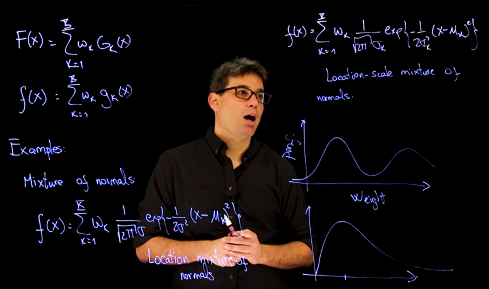
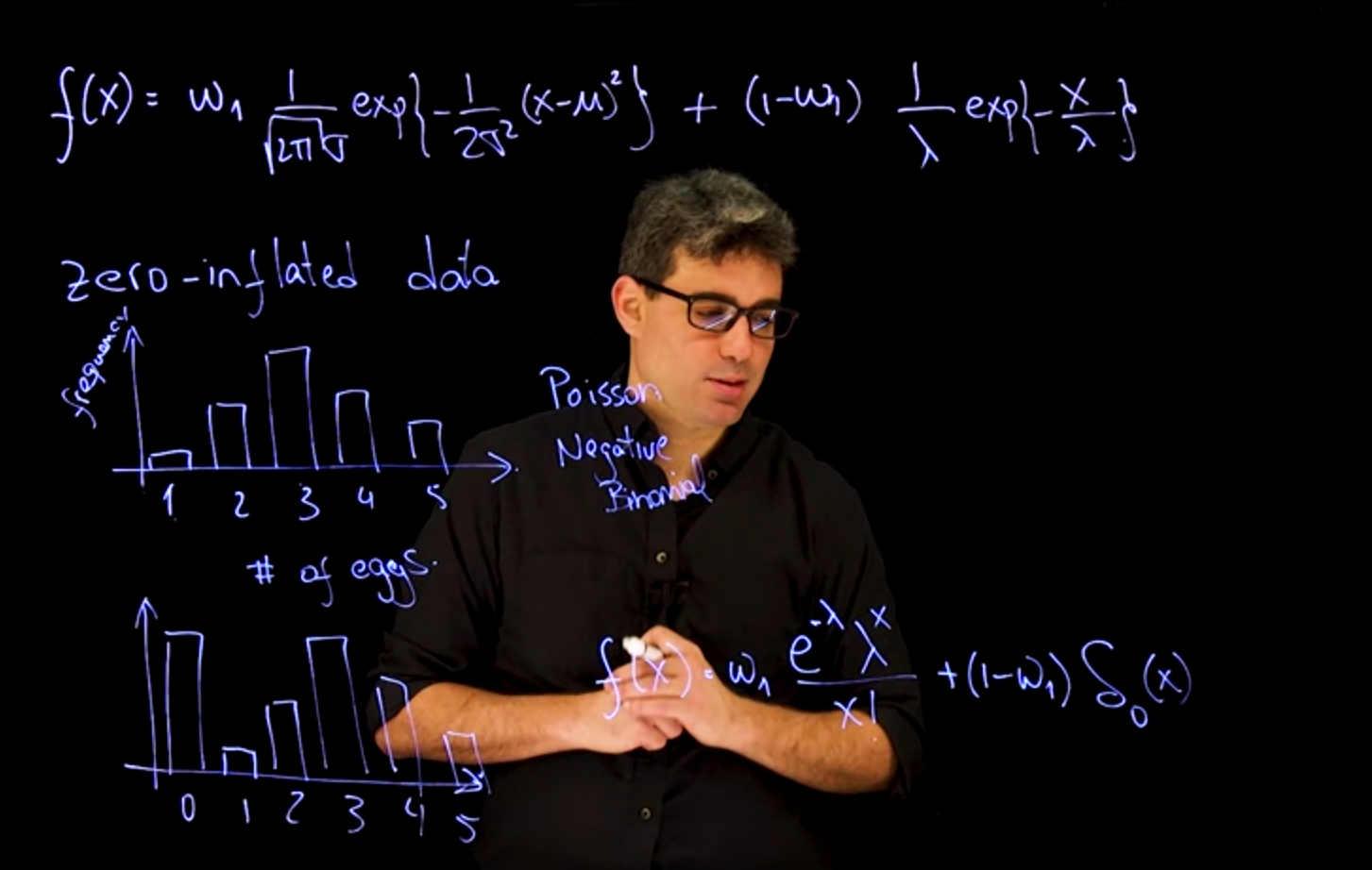
Example 55.2 (Location mixture of Normals)
f(x) = \sum_k \omega_k {1\over \sqrt{2 \pi \sigma}}e^{-{1\over 2 \sigma}(x-\mu_k)^2} \qquad \tag{55.5}
Example 55.3 (Location scale mixture of Normals)
f(x) = \sum_k \omega_k {1\over \sqrt{2 \pi \sigma_k}}e^{-{1\over 2 \sigma_k}(x-\mu_k)^2} \qquad \tag{55.6}
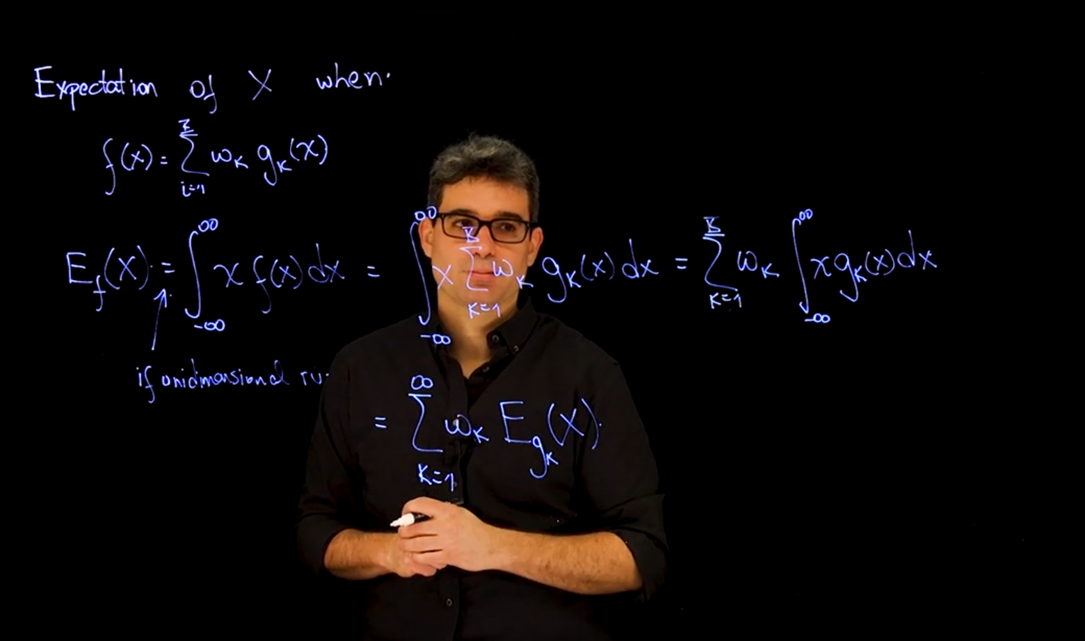
The expectation of a mixture is straightforward to compute, as it is a weighted sum of the expectations of the components.
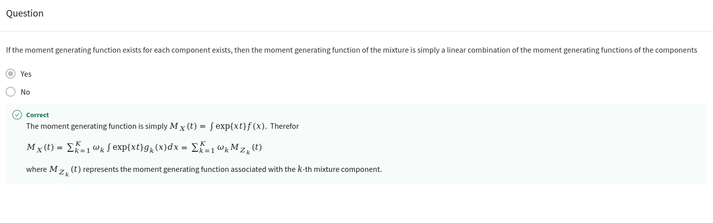
the moment generating function of a mixture is also straightforward to compute, as it is a weighted sum of the moment generating functions of the components.
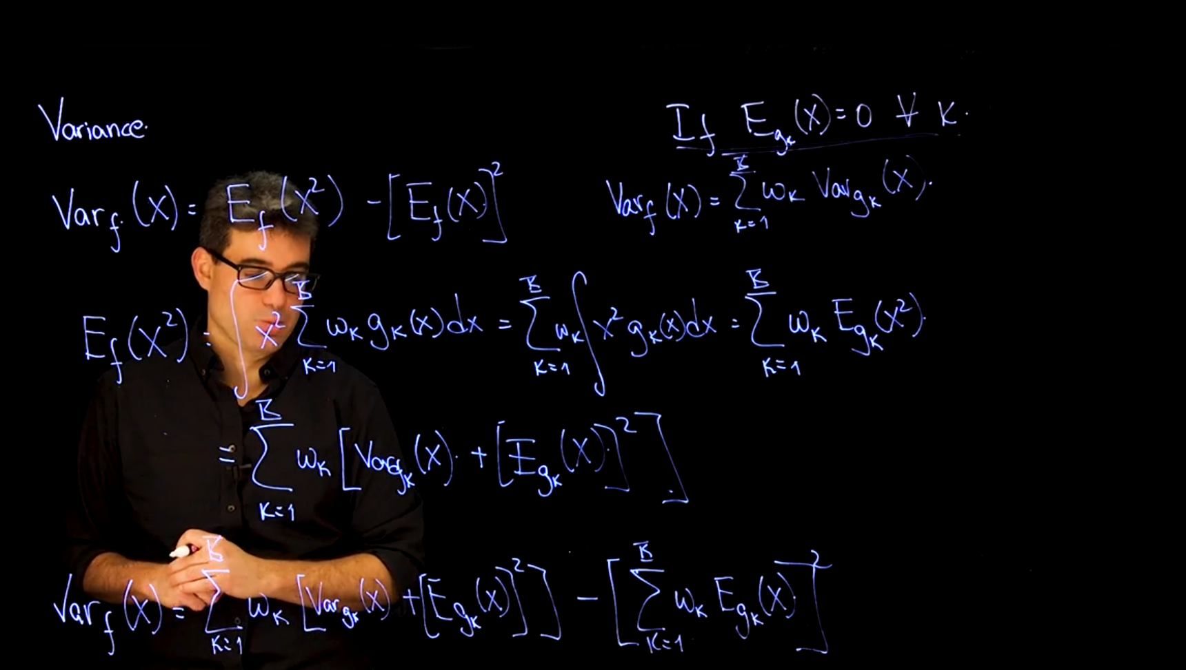
The variance of a mixture is not as straightforward to compute, as it involves the second moment of the components and the square of the expectation. However there is a degenerate case where the variance of the mixture is equal to the weighted sum of the variances of the components.
Here we will look at a few examples of mixtures of Gaussians which display different properties not available in a single Gaussian distribution. The video mostly walks through the code examples given in the readings below, while pointing out the features each of these mixtures possess that are not available in a single Gaussian distribution.
# Mixture of univariate Gaussians, bimodal
x = seq(-5, 12, length=100)
y = 0.6*dnorm(x, 0, 1) + 0.4*dnorm(x, 5, 2)
par(mar=c(4,4,1,1)+0.1)
plot(x, y, type="l", ylab="Density", las=1, lwd=2)
# set the title
title("Bimodal Mixture of Gaussians")# title: Mixture of univariate Gaussians, bimodal
from scipy.stats import norm
# Values to sample
x = np.linspace(-5, 12.0, num = 100)
# Normal 1 distribution
mu_1 = 0
std_1 = 1
r_n1 = norm.pdf(x,loc = mu_1, scale = std_1)
# Normal 2 Distribution
mu_2 = 5
std_2 = 2
r_n2 = norm.pdf(x, loc = mu_2, scale = std_2)
### computing mixture model
mixture_model = (0.6 * r_n1) + (0.4 * r_n2)
# Plotting the mixture models
fig, ax = plt.subplots(1, 1)
sns.lineplot(x=x, y=mixture_model)
plt.xlabel('Data')
plt.ylabel('Density')
plt.title('Mixture of two Gaussians')
plt.show()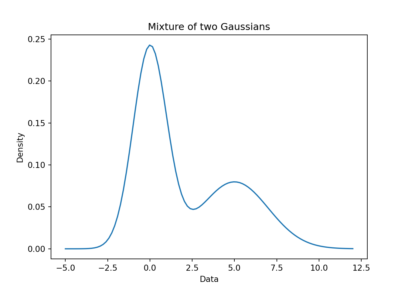
plt.close()f(x) = 0.55 \times \mathcal{N}(0, 2) + 0.45 \times \mathcal{N}(3, 4) \qquad \tag{55.7}
x = seq(-5, 12, length=100)
y = 0.55*dnorm(x, 0, sqrt(2)) + 0.45*dnorm(x, 3, 4)
par(mar=c(4,4,1,1)+0.1)
plot(x, y, type="l", ylab="Density", las=1, lwd=2)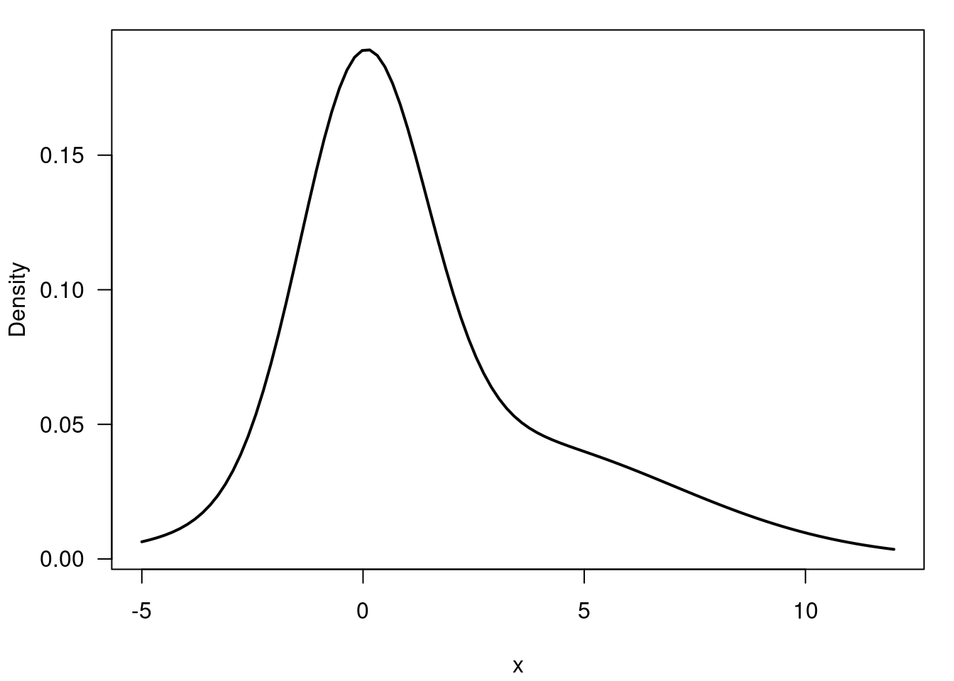
# Values to sample
x = np.linspace(-5, 12.0, num = 100)
# Normal 1 distribution
mu_1 = 0
var_1 = 2
r_n1 = norm.pdf(loc = mu_1, scale = np.sqrt(var_1), x = x)
# Normal 2 Distribution
mu_2 = 3
var_2 = 16
r_n2 = norm.pdf(loc = mu_2, scale = np.sqrt(var_2), x = x)

### computing mixture model
mixture_model = (0.55 * r_n1) + (0.45 * r_n2)

# Plotting the mixture models
fig, ax = plt.subplots(1, 1)
sns.lineplot(x=x, y=mixture_model)
plt.xlabel('Data')
plt.ylabel('Density')
plt.title('Mixture of two Gaussians Skewed')
plt.show()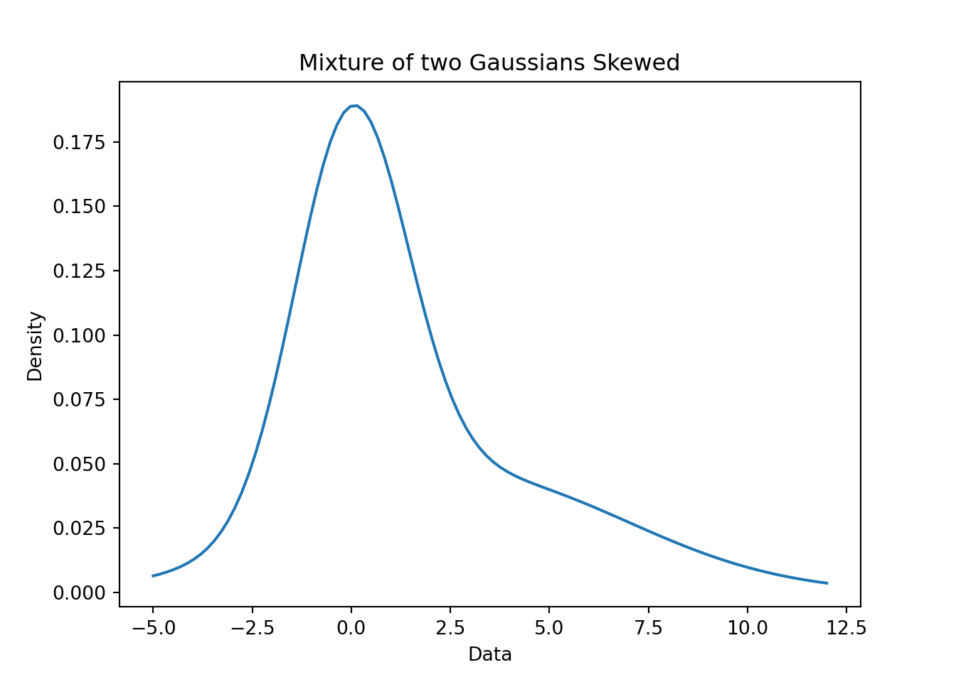
plt.close()f(x) = 0.40 \times \mathcal{N}(0, 2) + 0.40 \times \mathcal{N}(0, 4) + 0.20 \times \mathcal{N}(0, 5) \qquad \tag{55.8}
# simulate Mixture of univariate Gaussians, unimodal heavy tail

x = seq(-12, 12, length=100)
y = 0.40 * dnorm(x, 0, sqrt(2)) +
    0.40 * dnorm(x, 0, sqrt(16)) +
    0.20 * dnorm(x, 0, sqrt(20))
z = dnorm(x, 0, sqrt(0.4*2 + 0.4*16 + 0.2*20))par(mar=c(4,4,1,1)+0.1)
plot(x, y, type="l", ylab="Density", las=1, lwd=2)
lines(x, z, lty=2, lwd=2)
legend(2, 0.16, c("Mixture","Gaussian"), lty=c(1,2), bty="n", cex=0.77, lwd=c(2,2))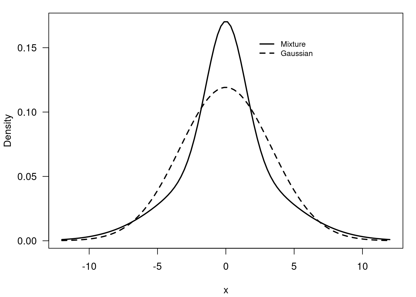
# Values to sample
x = np.linspace(-12.0, 12.0, num = 100)
# Normal 1 distribution
mu_1 = 0
var_1 = 2
r_n1 = norm.pdf(loc = mu_1, scale = np.sqrt(var_1), x = x)
# Normal 2 Distribution
mu_2 = 0
var_2 = 16
r_n2 = norm.pdf(loc = mu_2, scale = np.sqrt(var_2), x = x)
# Normal 3 Distribution
mu_3 = 0
var_3 = 20
r_n3 = norm.pdf(loc = mu_3, scale = np.sqrt(var_3), x = x)

### computing mixture model
y = (0.4 * r_n1) + (0.4 * r_n2) + (0.2 * r_n3)
z = norm.pdf(loc = 0, scale = np.sqrt(0.4 * 2 + 0.4 * 16 + 0.2 * 20), x = x)
# Plotting the mixture models
fig, ax = plt.subplots(1, 1)
sns.lineplot(x=x, y=y)
ax.plot(x, z, '--')
plt.xlabel('Data')
plt.ylabel('Density')
plt.title('Mixture of gaussians heavy tailed')
plt.legend(['Mixture', 'Gaussian'])
plt.show()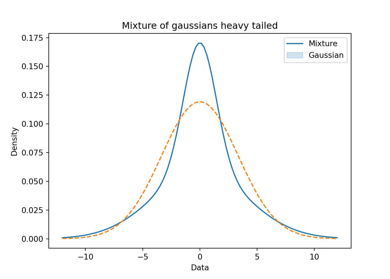
plt.close()
Note there are two approaches to zero inflation:
This is a mixture of a point mass at zero and a log Gaussian distribution. This corresponds to the example where we have a light bulb factory and we want to model the time to failure of the light bulbs. We know that for the defective light bulbs, the time to failure is zero. For the non-defective light bulbs, the time to failure is log normally distributed with mean 1.5 and standard deviation 0.5
f(x) = 0.3 \times \mathbb{I}_{x\ge0} + 0.7 \times \mathcal{LN}(1.5, 0.5) \qquad \tag{55.9}
## The ZILN model
x = seq(-2, 15, length=1000)
y = plnorm(x, 1.5, 0.5)
z = 0.3*as.numeric(x>=0) + (1-0.3)*y
## The plot
par(mar=c(4,4,1,1)+0.1)
plot(x, y, type="l", las=1, lty=2, xlab="x",
ylab="Cumulative distribution Function", lwd=2)
lines(x, z, lty=1, lwd=2)
legend(4, 0.45, c("Zero infla. log Gaussian","log Gaussian"),
lty=c(1,2), bty="n", lwd=c(2,2))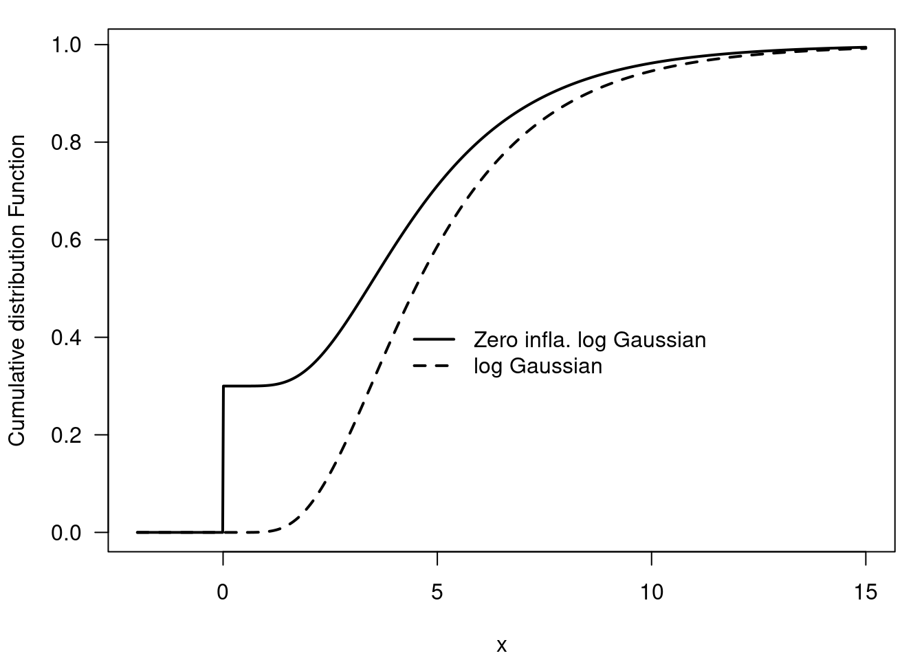
import numpy as np
import matplotlib.pyplot as plt
from scipy.stats import lognorm

# Zero-inflated continuous distribution
# Values to sample
x = np.linspace(-2.0, 15.0, num = 200)
# See for parameterization
y = lognorm.pdf(loc = 0, scale = np.exp(1.5), s = 0.5, x = x)

# Point mass vector
p_mass = np.zeros(len(x))
p_mass[x >= 0] = 1
z = 0.3 * p_mass + (1 - 0.3) * y
## title: Zero inflated negative binomial distribution
# Plotting the mixture models
fig, ax = plt.subplots(1, 1)
ax.plot(x, y)
ax.plot(x, z, '--')
plt.xlabel('X')
plt.ylabel('Cumulative distribution function')
plt.title('Zero-inflated continuous distribution')
plt.legend(['Log gaussian', 'Zero infla. Log gaussian'])
plt.show()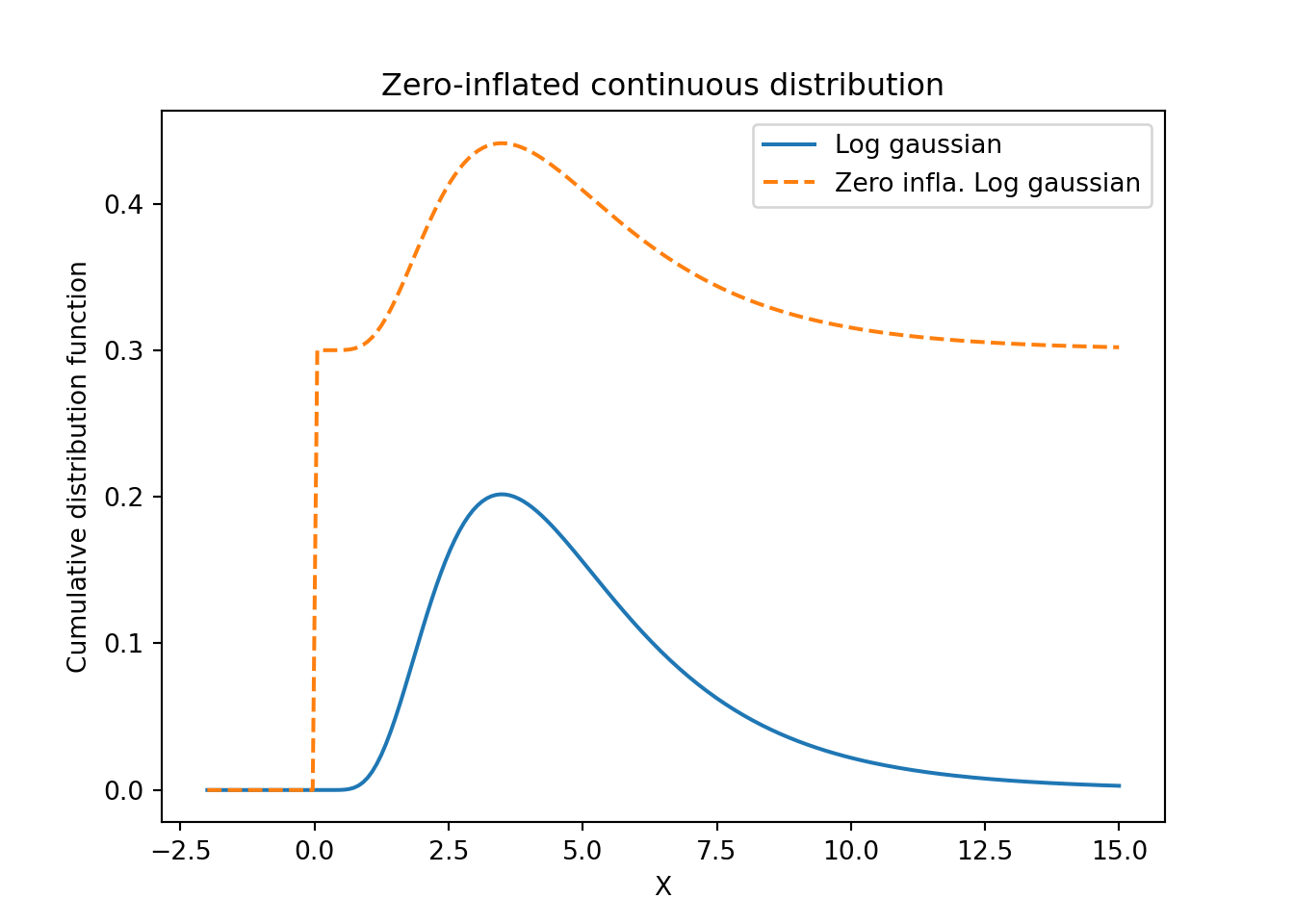
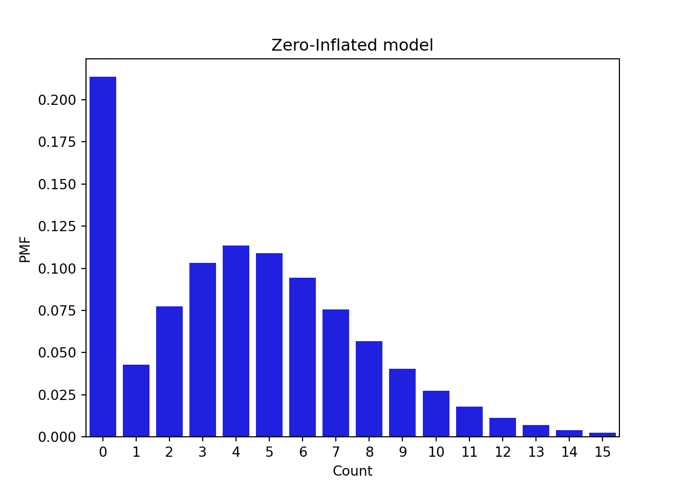
f(x) = 0.2 \times \mathbb{I}_{x=0} + 0.8 \times NB(8, 0.6) \qquad \tag{55.10}
## title: Zero inflated negative binomial distribution
x = seq(0, 15)
y = dnbinom(x, 8, 0.6)
z = 0.2*c(1,rep(0,length(x)-1)) + (1-0.2)*y
par(mfrow=c(2,1))
par(mar=c(4,4,2,2)+0.1)
barplot(y, names.arg=x, las=1, xlab = "x", ylab="Probability",
        border=NA, main="Negative Binomial")
par(mar=c(4,4,1,1)+0.1)
barplot(z, names.arg=x, las=1, xlab = "x", ylab="Probability",
        border=NA, main="Zero-inflated Negative Binomial")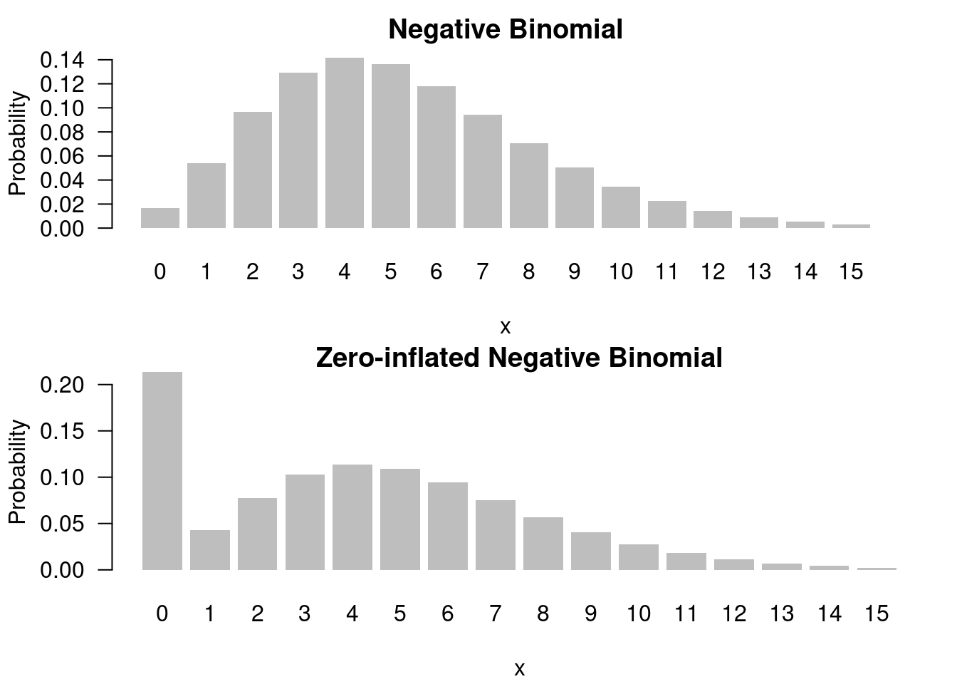
## title: Zero inflated negative binomial distribution
from scipy.stats import nbinom
import seaborn as sns

# Values to sample
x = np.arange(0, 16)
y = nbinom.pmf(x, n = 8, p = 0.6)

# Plotting the negative binomial model
fig, ax = plt.subplots(1, 1)

sns.barplot(x=x, y=y, color = 'blue')

plt.title('Negative Binomial')
plt.xlabel('Count')
plt.ylabel('PMF')
plt.show()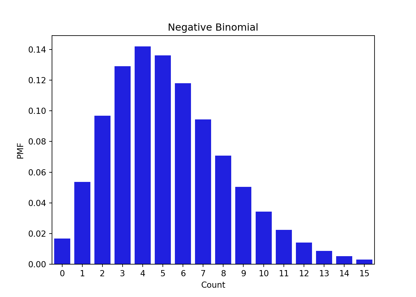
# Point mass vector
p_mass = np.zeros(len(x))
p_mass[0] = 1
z = 0.2 * p_mass + (1 - 0.2) * y

# Plotting the zero-inflated model
fig, ax = plt.subplots(1, 1)
sns.barplot(x=x, y=z, color = 'blue')
plt.title('Zero-Inflated model')
plt.xlabel('Count')
plt.ylabel('PMF')
plt.show()