data("PlantGrowth")
#?PlantGrowth
head(PlantGrowth)
weight group
1 4.17 ctrl
2 5.58 ctrl
3 5.18 ctrl
4 6.11 ctrl
5 4.50 ctrl
6 4.61 ctrlANOVA, Bayesian statistics, R programming, statistical modeling, Analysis of Variance
As an example of a one-way ANOVA, we’ll look at the Plant Growth data in R.
data("PlantGrowth")
#?PlantGrowth
head(PlantGrowth) weight group
1 4.17 ctrl
2 5.58 ctrl
3 5.18 ctrl
4 6.11 ctrl
5 4.50 ctrl
6 4.61 ctrlWe first load the dataset (Listing 43.1)
Because the explanatory variable group is a factor and not continuous, we choose to visualize the data with box plots rather than scatter plots.
boxplot(weight ~ group, data=PlantGrowth)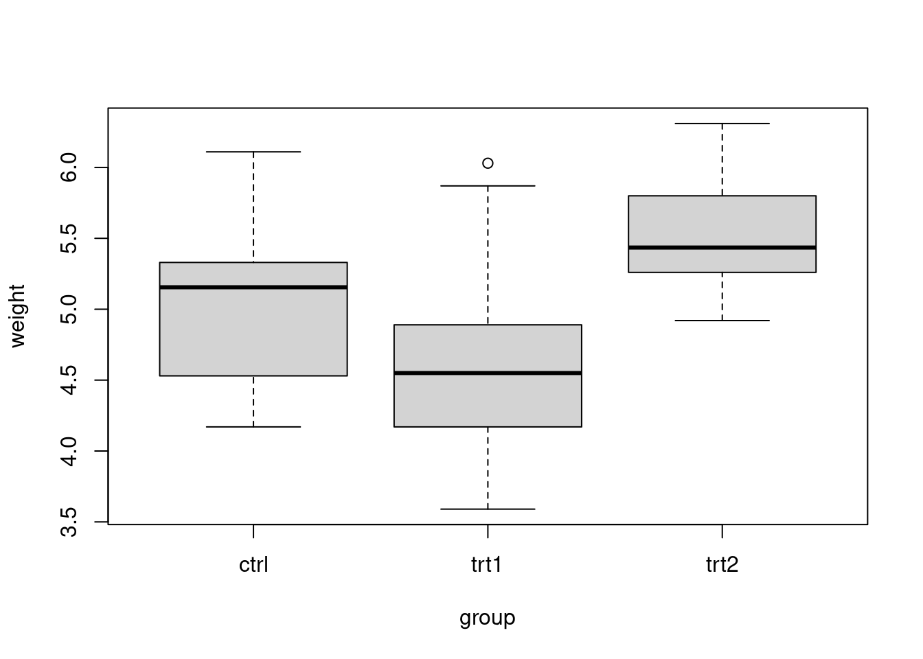
The box plots summarize the distribution of the data for each of the three groups. It appears that treatment 2 has the highest mean yield. It might be questionable whether each group has the same variance, but we’ll assume that is the case.
Again, we can start with the reference analysis (with a noninformative prior) with a linear model in R.
lmod = lm(weight ~ group, data=PlantGrowth)
summary(lmod)
Call:
lm(formula = weight ~ group, data = PlantGrowth)

Residuals:
    Min      1Q  Median      3Q     Max
-1.0710 -0.4180 -0.0060  0.2627  1.3690

Coefficients:
            Estimate Std. Error t value Pr(>|t|)
(Intercept)   5.0320     0.1971  25.527   <2e-16 ***
grouptrt1    -0.3710     0.2788  -1.331   0.1944
grouptrt2     0.4940     0.2788   1.772   0.0877 .
---
Signif. codes:  0 '***' 0.001 '**' 0.01 '*' 0.05 '.' 0.1 ' ' 1

Residual standard error: 0.6234 on 27 degrees of freedom
Multiple R-squared:  0.2641,    Adjusted R-squared:  0.2096
F-statistic: 4.846 on 2 and 27 DF, p-value: 0.01591anova(lmod)Analysis of Variance Table
Response: weight
Df Sum Sq Mean Sq F value Pr(>F)
group 2 3.7663 1.8832 4.8461 0.01591 *
Residuals 27 10.4921 0.3886
---
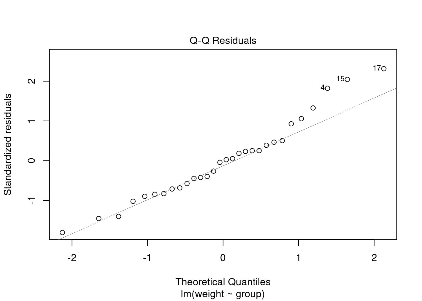
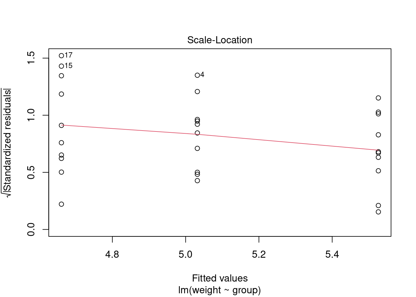
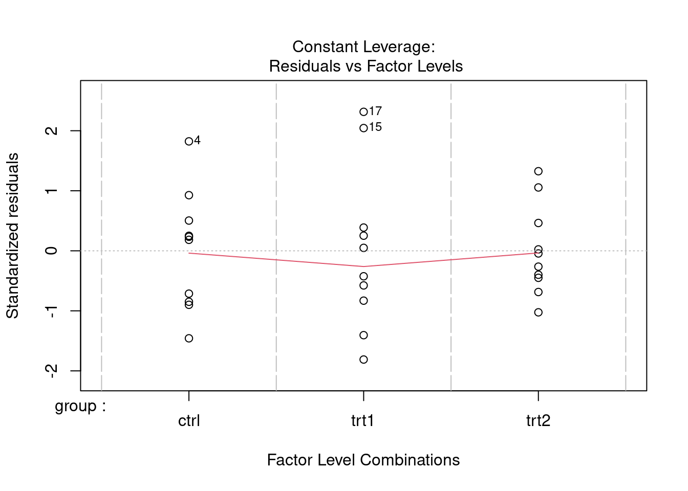
Signif. codes: 0 '***' 0.001 '**' 0.01 '*' 0.05 '.' 0.1 ' ' 1plot(lmod) # for graphical residual analysis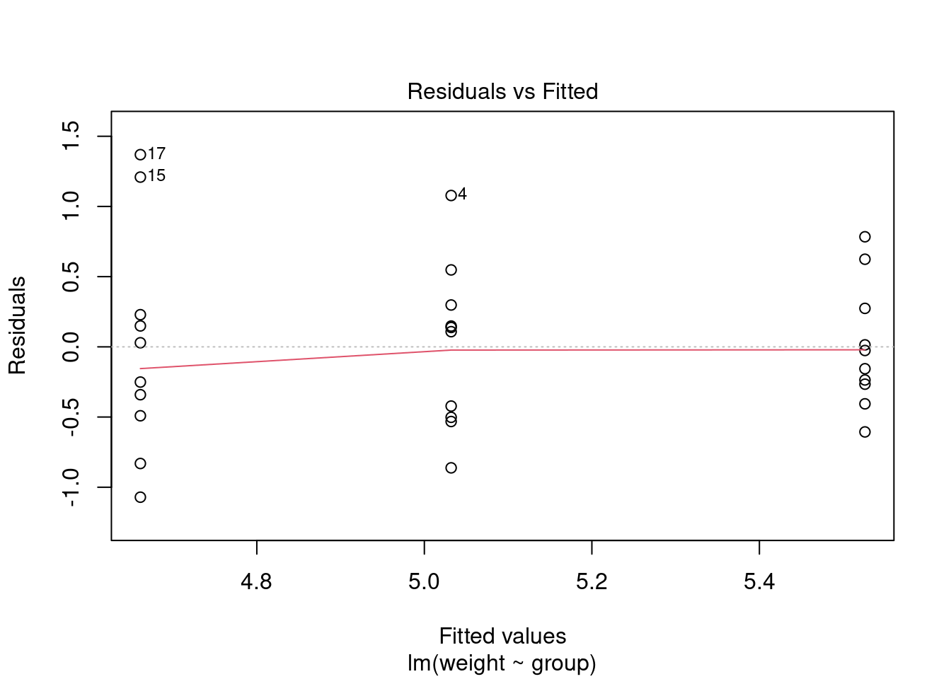
The default model structure in R is the linear model with dummy indicator variables. Hence, the “intercept” in this model is the mean yield for the control group. The two other parameters are the estimated effects of treatments 1 and 2. To recover the mean yield in treatment group 1, you would add the intercept term and the treatment 1 effect. To see how R sets the model up, use the model.matrix(lmod) function to extract the X matrix.
The anova() function in R compares variability of observations between the treatment groups to variability within the treatment groups to test whether all means are equal or whether at least one is different. The small p-value here suggests that the means are not all equal.
Let’s fit the cell means model in JAGS.
library("rjags")mod_string = " model {
for (i in 1:length(y)) {
y[i] ~ dnorm(mu[grp[i]], prec)
}
for (j in 1:3) {
mu[j] ~ dnorm(0.0, 1.0/1.0e6)
}
prec ~ dgamma(5/2.0, 5*1.0/2.0)
sig = sqrt( 1.0 / prec )
} "
set.seed(82)
str(PlantGrowth)'data.frame': 30 obs. of 2 variables:
$ weight: num 4.17 5.58 5.18 6.11 4.5 4.61 5.17 4.53 5.33 5.14 ...
$ group : Factor w/ 3 levels "ctrl","trt1",..: 1 1 1 1 1 1 1 1 1 1 ...data_jags = list(y=PlantGrowth$weight,
grp=as.numeric(PlantGrowth$group))
params = c("mu", "sig")
inits = function() {
inits = list("mu"=rnorm(3,0.0,100.0), "prec"=rgamma(1,1.0,1.0))
}
mod = jags.model(textConnection(mod_string), data=data_jags, inits=inits, n.chains=3)Compiling model graph
Resolving undeclared variables
Allocating nodes
Graph information:
Observed stochastic nodes: 30
Unobserved stochastic nodes: 4
Total graph size: 74
Initializing modelupdate(mod, 1e3)
mod_sim = coda.samples(model=mod,
variable.names=params,
n.iter=5e3)
mod_csim = as.mcmc(do.call(rbind, mod_sim)) # combined chainsAs usual, we check for convergence of our MCMC.
par(mar = c(2.5, 1, 2.5, 1))
plot(mod_sim)

gelman.diag(mod_sim)
Potential scale reduction factors:
Point est. Upper C.I.
mu[1] 1 1
mu[2] 1 1
mu[3] 1 1
sig 1 1
Multivariate psrf
1autocorr.diag(mod_sim) mu[1] mu[2] mu[3] sig
Lag 0 1.000000000 1.0000000000 1.000000000 1.000000000
Lag 1 -0.011460881 0.0024771025 -0.004490544 0.091526162
Lag 5 0.004808698 -0.0028043283 -0.003078623 -0.003216494
Lag 10 -0.003905758 -0.0006634477 0.007273004 0.006594108
Lag 50 -0.005396650 -0.0147926765 0.001604061 -0.006288827effectiveSize(mod_sim) mu[1] mu[2] mu[3] sig
15264.43 14972.85 15000.00 12780.55 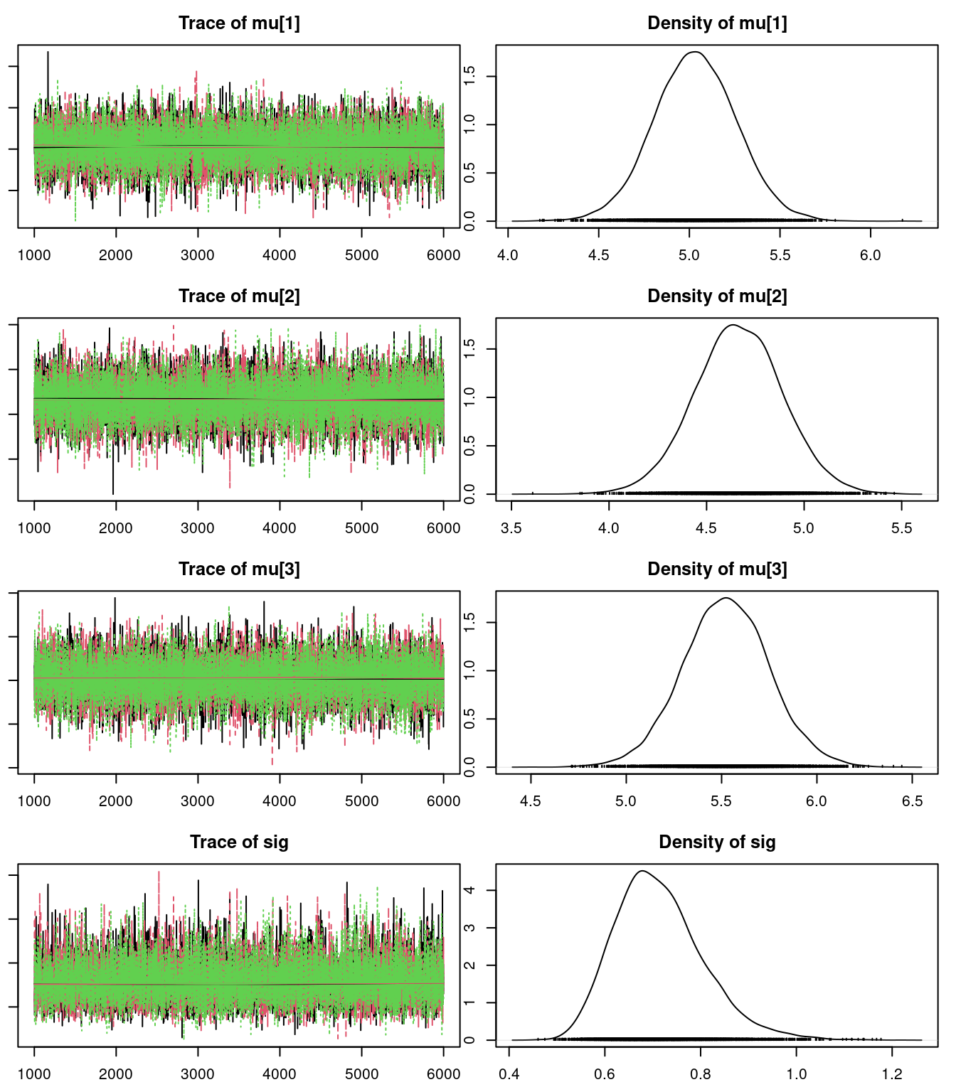
We can also look at the residuals to see if there are any obvious problems with our model choice.
(pm_params = colMeans(mod_csim)) mu[1] mu[2] mu[3] sig
5.0293601 4.6641252 5.5276317 0.7138066 yhat = pm_params[1:3][data_jags$grp]
resid = data_jags$y - yhat
plot(resid)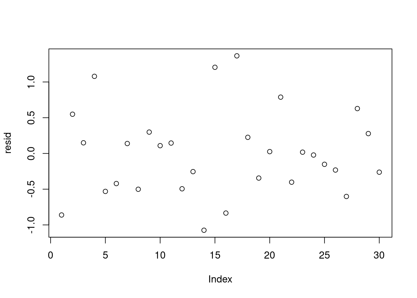
plot(yhat, resid)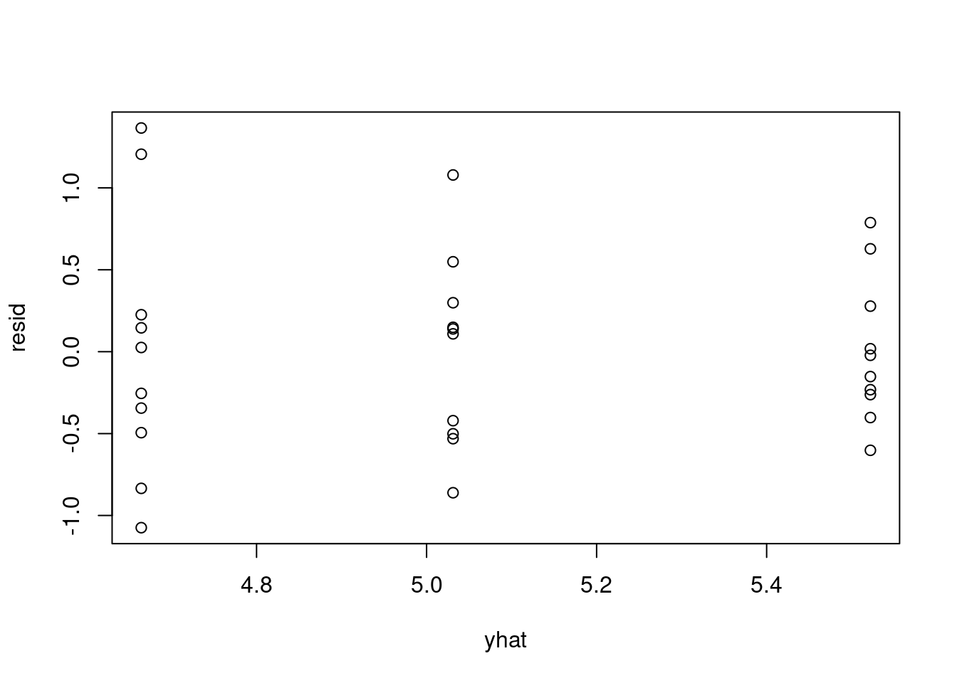
Again, it might be appropriate to have a separate variance for each group. We will have you do that as an exercise.
Let’s look at the posterior summary of the parameters.
summary(mod_sim)
Iterations = 1001:6000
Thinning interval = 1
Number of chains = 3
Sample size per chain = 5000

1. Empirical mean and standard deviation for each variable,
   plus standard error of the mean:

        Mean      SD  Naive SE Time-series SE
mu[1] 5.0294 0.22845 0.0018653      0.0018495
mu[2] 4.6641 0.22831 0.0018642      0.0018671
mu[3] 5.5276 0.22713 0.0018545      0.0018546
sig   0.7138 0.09181 0.0007496      0.0008137

2. Quantiles for each variable:

        2.5%    25%    50%    75%  97.5%
mu[1] 4.5787 4.8814 5.0280 5.1776 5.4851
mu[2] 4.2164 4.5115 4.6633 4.8159 5.1066
mu[3] 5.0795 5.3774 5.5306 5.6763 5.9696
sig 0.5611 0.6495 0.7039 0.7679 0.9219HPDinterval(mod_csim) lower upper
mu[1] 4.580084 5.4867523
mu[2] 4.214417 5.1037609
mu[3] 5.070161 5.9587615
sig 0.544779 0.8946966
attr(,"Probability")
[1] 0.95The HPDinterval() function in the coda package calculates intervals of highest posterior density for each parameter.
We are interested to know if one of the treatments increases mean yield. It is clear that treatment 1 does not. What about treatment 2?
mean(mod_csim[,3] > mod_csim[,1])[1] 0.9388There is a high posterior probability that the mean yield for treatment 2 is greater than the mean yield for the control group.
It may be the case that treatment 2 would be costly to put into production. Suppose that to be worthwhile, this treatment must increase mean yield by 10%. What is the posterior probability that the increase is at least that?
mean(mod_csim[,3] > 1.1*mod_csim[,1])[1] 0.4952We have about 50/50 odds that adopting treatment 2 would increase mean yield by at least 10%.
Let’s explore an example with two factors. We’ll use the Warpbreaks data set in R. Check the documentation for a description of the data by typing ?warpbreaks.
data("warpbreaks")
#?warpbreaks
head(warpbreaks)
breaks wool tension
1 26 A L
2 30 A L
3 54 A L
4 25 A L
5 70 A L
6 52 A L# This chunk is for displaying the output that was previously static.
# If the static output below is preferred, this chunk can be removed
# and the static output remains unlabelled as it's not a code cell.
# For a labeled table, this chunk should generate it.
# The original file had static output here:
## breaks wool tension
## 1 26 A L
## 2 30 A L
## 3 54 A L
## 4 25 A L
## 5 70 A L
## 6 52 A L
# To make this a labeled table from code:
head(warpbreaks) breaks wool tension
1 26 A L
2 30 A L
3 54 A L
4 25 A L
5 70 A L
6 52 A Ltable(warpbreaks$wool, warpbreaks$tension)
    L M H
  A 9 9 9
  B 9 9 9
Again, we visualize the data with box plots.
boxplot(breaks ~ wool + tension, data=warpbreaks)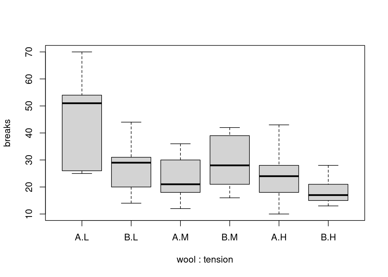
boxplot(log(breaks) ~ wool + tension, data=warpbreaks)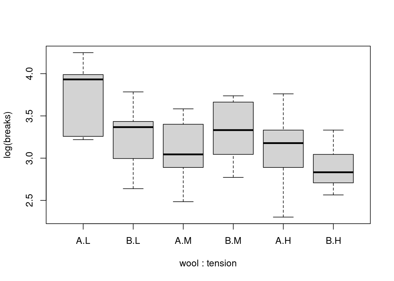
The different groups have more similar variance if we use the logarithm of breaks. From this visualization, it looks like both factors may play a role in the number of breaks. It appears that there is a general decrease in breaks as we move from low to medium to high tension. Let’s start with a one-way model using tension only.
mod1_string = " model {
    for( i in 1:length(y)) {
        y[i] ~ dnorm(mu[tensGrp[i]], prec)
    }

    for (j in 1:3) {
        mu[j] ~ dnorm(0.0, 1.0/1.0e6)
    }

    prec ~ dgamma(5/2.0, 5*2.0/2.0)
    sig = sqrt(1.0 / prec)
} "

set.seed(83)
str(warpbreaks)
'data.frame': 54 obs. of 3 variables:
$ breaks : num 26 30 54 25 70 52 51 26 67 18 ...
$ wool : Factor w/ 2 levels "A","B": 1 1 1 1 1 1 1 1 1 1 ...
$ tension: Factor w/ 3 levels "L","M","H": 1 1 1 1 1 1 1 1 1 2 ...data1_jags = list(y=log(warpbreaks$breaks), tensGrp=as.numeric(warpbreaks$tension))
params1 = c("mu", "sig")
mod1 = jags.model(textConnection(mod1_string), data=data1_jags, n.chains=3)Compiling model graph
Resolving undeclared variables
Allocating nodes
Graph information:
Observed stochastic nodes: 54
Unobserved stochastic nodes: 4
Total graph size: 123
Initializing modelupdate(mod1, 1e3)
mod1_sim = coda.samples(model=mod1,
variable.names=params1,
n.iter=5e3)## convergence diagnostics
plot(mod1_sim)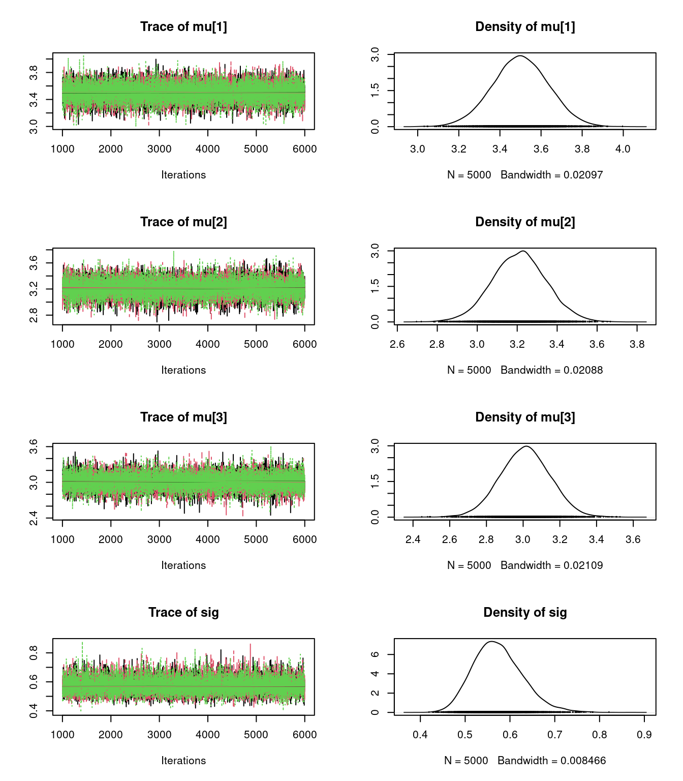
gelman.diag(mod1_sim)Potential scale reduction factors:
Point est. Upper C.I.
mu[1] 1 1
mu[2] 1 1
mu[3] 1 1
sig 1 1
Multivariate psrf
1autocorr.diag(mod1_sim) mu[1] mu[2] mu[3] sig
Lag 0 1.0000000000 1.000000000 1.000000000 1.000000000
Lag 1 -0.0093994624 -0.006129630 0.005427660 0.059615763
Lag 5 -0.0005895951 0.007676833 -0.004840208 0.001066727
Lag 10 -0.0013471491 0.007570268 -0.005143937 0.009405400
Lag 50 -0.0176327412 0.004889020 -0.006431633 -0.012297885effectiveSize(mod1_sim) mu[1] mu[2] mu[3] sig
15000.00 15000.00 15000.00 13114.96 The 95% posterior interval for the mean of group 2 (medium tension) overlaps with both the low and high groups, but the intervals for low and high group only slightly overlap. That is a pretty strong indication that the means for low and high tension are different. Let’s collect the DIC for this model and move on to the two-way model.
dic1 = dic.samples(mod1, n.iter=1e3)With two factors, one with two levels and the other with three, we have six treatment groups, which is the same situation we discussed when introducing multiple factor ANOVA. We will first fit the additive model which treats the two factors separately with no interaction. To get the X matrix (or design matrix) for this model, we can create it in R.
X = model.matrix( ~ wool + tension, data=warpbreaks)
head(X)
(Intercept) woolB tensionM tensionH
1 1 0 0 0
2 1 0 0 0
3 1 0 0 0
4 1 0 0 0
5 1 0 0 0
6 1 0 0 0tail(X) (Intercept) woolB tensionM tensionH
49 1 1 0 1
50 1 1 0 1
51 1 1 0 1
52 1 1 0 1
53 1 1 0 1
54 1 1 0 1By default, R has chosen the mean for wool A and low tension to be the intercept. Then, there is an effect for wool B, and effects for medium tension and high tension, each associated with dummy indicator variables.
mod2_string = " model {
    for( i in 1:length(y)) {
        y[i] ~ dnorm(mu[i], prec)
        mu[i] = int + alpha*isWoolB[i] + beta[1]*isTensionM[i] + beta[2]*isTensionH[i]
    }

    int ~ dnorm(0.0, 1.0/1.0e6)
    alpha ~ dnorm(0.0, 1.0/1.0e6)
    for (j in 1:2) {
        beta[j] ~ dnorm(0.0, 1.0/1.0e6)
    }

    prec ~ dgamma(3/2.0, 3*1.0/2.0)
    sig = sqrt(1.0 / prec)
} "

data2_jags = list(y=log(warpbreaks$breaks), isWoolB=X[,"woolB"], isTensionM=X[,"tensionM"], isTensionH=X[,"tensionH"])

params2 = c("int", "alpha", "beta", "sig")

mod2 = jags.model(textConnection(mod2_string), data=data2_jags, n.chains=3)
Compiling model graph
Resolving undeclared variables
Allocating nodes
Graph information:
Observed stochastic nodes: 54
Unobserved stochastic nodes: 5
Total graph size: 243
Initializing modelupdate(mod2, 1e3)
mod2_sim = coda.samples(model=mod2,
variable.names=params2,
n.iter=5e3)## convergence diagnostics
plot(mod2_sim)
gelman.diag(mod2_sim) # Corrected from mod1_simPotential scale reduction factors:
Point est. Upper C.I.
alpha 1 1
beta[1] 1 1
beta[2] 1 1
int 1 1
sig 1 1
Multivariate psrf
1autocorr.diag(mod2_sim) # Corrected from mod1_sim alpha beta[1] beta[2] int sig
Lag 0 1.000000000 1.000000000 1.000000000 1.00000000 1.000000000
Lag 1 0.504604466 0.511981569 0.498469114 0.74838601 0.085720291
Lag 5 0.031190681 0.102428217 0.119526968 0.19519879 0.011414612
Lag 10 0.010485978 0.015627274 0.021627102 0.04149613 -0.009831302
Lag 50 -0.009020857 -0.007539669 -0.005953837 -0.01208873 0.001180826effectiveSize(mod2_sim) # Corrected from mod1_sim alpha beta[1] beta[2] int sig
5037.651 3778.790 3407.480 2326.049 12221.326 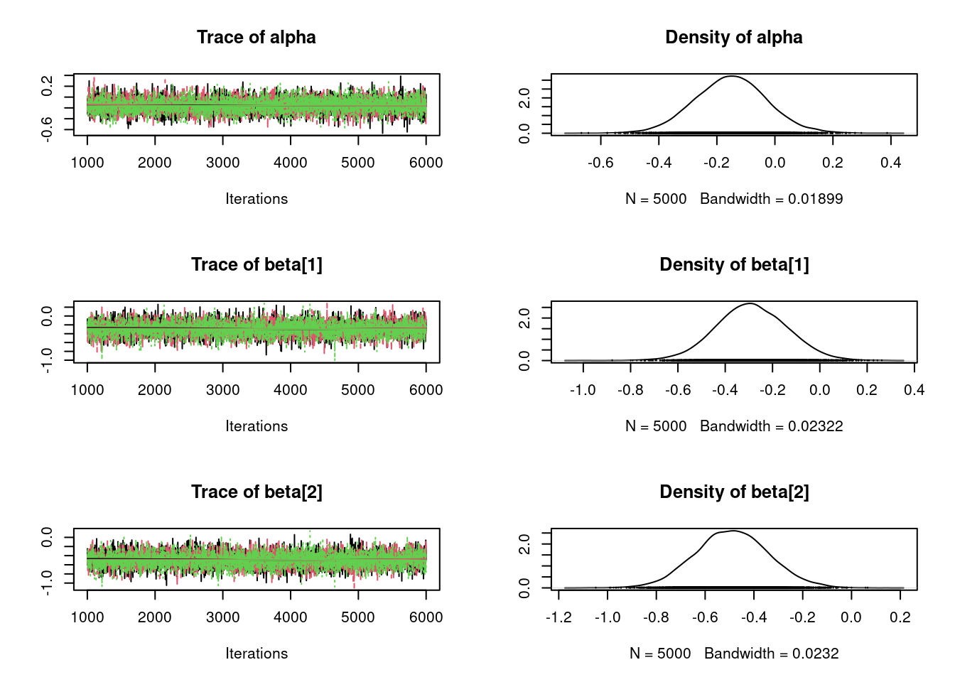
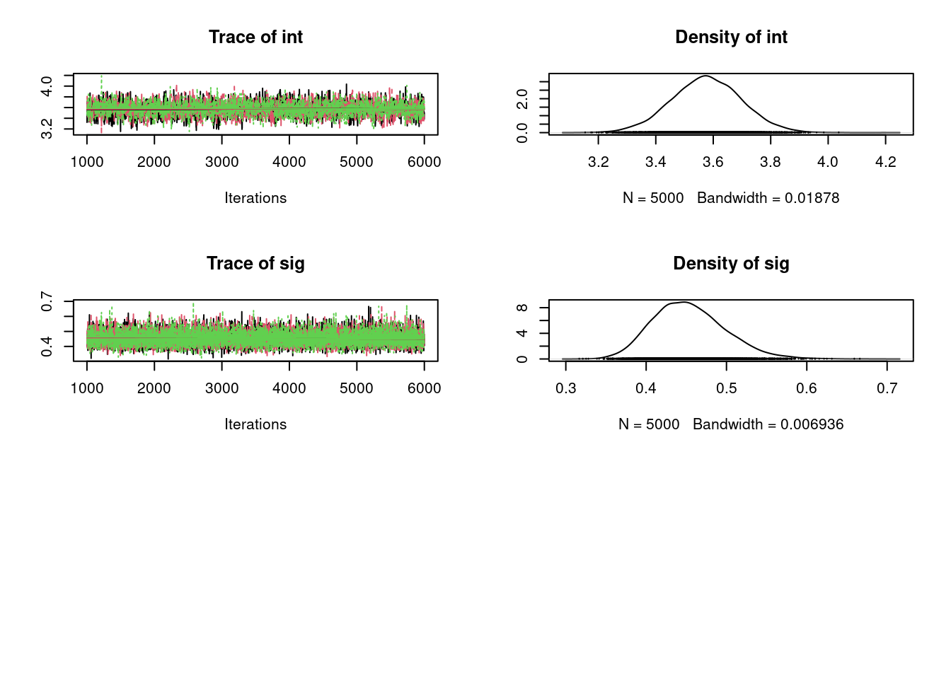
Let’s summarize the results, collect the DIC for this model, and compare it to the first one-way model.
summary(mod2_sim)
Iterations = 1001:6000
Thinning interval = 1
Number of chains = 3
Sample size per chain = 5000

1. Empirical mean and standard deviation for each variable,
   plus standard error of the mean:

           Mean      SD  Naive SE Time-series SE
alpha   -0.1544 0.12515 0.0010218      0.0017634
beta[1] -0.2897 0.15409 0.0012581      0.0025097
beta[2] -0.4898 0.15164 0.0012381      0.0026060
int      3.5788 0.12422 0.0010143      0.0025762
sig      0.4546 0.04501 0.0003675      0.0004074

2. Quantiles for each variable:

           2.5%     25%     50%      75%     97.5%
alpha   -0.4066 -0.2364 -0.1541 -0.06956  0.085274
beta[1] -0.5940 -0.3920 -0.2881 -0.18716  0.009971
beta[2] -0.7899 -0.5898 -0.4896 -0.38859 -0.192792
int      3.3387  3.4951  3.5779  3.65983  3.827696
sig 0.3765 0.4231 0.4508 0.48233 0.553702(dic2 = dic.samples(mod2, n.iter=1e3))Mean deviance: 55.51
penalty 5.074
Penalized deviance: 60.58 dic1Mean deviance: 66.47
penalty 4.026
Penalized deviance: 70.5 This suggests there is much to be gained adding the wool factor to the model. Before we settle on this model however, we should consider whether there is an interaction. Let’s look again at the box plot with all six treatment groups.
boxplot(log(breaks) ~ wool + tension, data=warpbreaks)
Our two-way model has a single effect for wool B and the estimate is negative. If this is true, then we would expect wool B to be associated with fewer breaks than its wool A counterpart on average. This is true for low and high tension, but it appears that breaks are higher for wool B when there is medium tension. That is, the effect for wool B is not consistent across tension levels, so it may appropriate to add an interaction term. In R, this would look like:
lmod2 = lm(log(breaks) ~ .^2, data=warpbreaks)
summary(lmod2)
Call:
lm(formula = log(breaks) ~ .^2, data = warpbreaks)

Residuals:
     Min       1Q   Median       3Q      Max
-0.81504 -0.27885  0.04042  0.27319  0.64358

Coefficients:
               Estimate Std. Error t value Pr(>|t|)
(Intercept)      3.7179     0.1247  29.824  < 2e-16 ***
woolB           -0.4356     0.1763  -2.471  0.01709 *
tensionM        -0.6012     0.1763  -3.410  0.00133 **
tensionH        -0.6003     0.1763  -3.405  0.00134 **
woolB:tensionM   0.6281     0.2493   2.519  0.01514 *
woolB:tensionH   0.2221     0.2493   0.891  0.37749
---
Signif. codes:  0 '***' 0.001 '**' 0.01 '*' 0.05 '.' 0.1 ' ' 1

Residual standard error: 0.374 on 48 degrees of freedom
Multiple R-squared:  0.3363,    Adjusted R-squared:  0.2672
F-statistic: 4.864 on 5 and 48 DF,  p-value: 0.001116
Adding the interaction, we get an effect for being in wool B and medium tension, as well as for being in wool B and high tension. There are now six parameters for the mean, one for each treatment group, so this model is equivalent to the full cell means model. Let’s use that.
In this new model, \mu will be a matrix with six entries, each corresponding to a treatment group.
mod3_string = " model {
    for( i in 1:length(y)) {
        y[i] ~ dnorm(mu[woolGrp[i], tensGrp[i]], prec)
    }

    for (j in 1:max(woolGrp)) {
        for (k in 1:max(tensGrp)) {
            mu[j,k] ~ dnorm(0.0, 1.0/1.0e6)
        }
    }

    prec ~ dgamma(3/2.0, 3*1.0/2.0)
    sig = sqrt(1.0 / prec)
} "

str(warpbreaks)
'data.frame': 54 obs. of 3 variables:
$ breaks : num 26 30 54 25 70 52 51 26 67 18 ...
$ wool : Factor w/ 2 levels "A","B": 1 1 1 1 1 1 1 1 1 1 ...
$ tension: Factor w/ 3 levels "L","M","H": 1 1 1 1 1 1 1 1 1 2 ...data3_jags = list(y=log(warpbreaks$breaks), woolGrp=as.numeric(warpbreaks$wool), tensGrp=as.numeric(warpbreaks$tension))
params3 = c("mu", "sig")
mod3 = jags.model(textConnection(mod3_string), data=data3_jags, n.chains=3)Compiling model graph
Resolving undeclared variables
Allocating nodes
Graph information:
Observed stochastic nodes: 54
Unobserved stochastic nodes: 7
Total graph size: 179
Initializing modelupdate(mod3, 1e3)
mod3_sim = coda.samples(model=mod3,
variable.names=params3,
n.iter=5e3)
mod3_csim = as.mcmc(do.call(rbind, mod3_sim))plot(mod3_sim)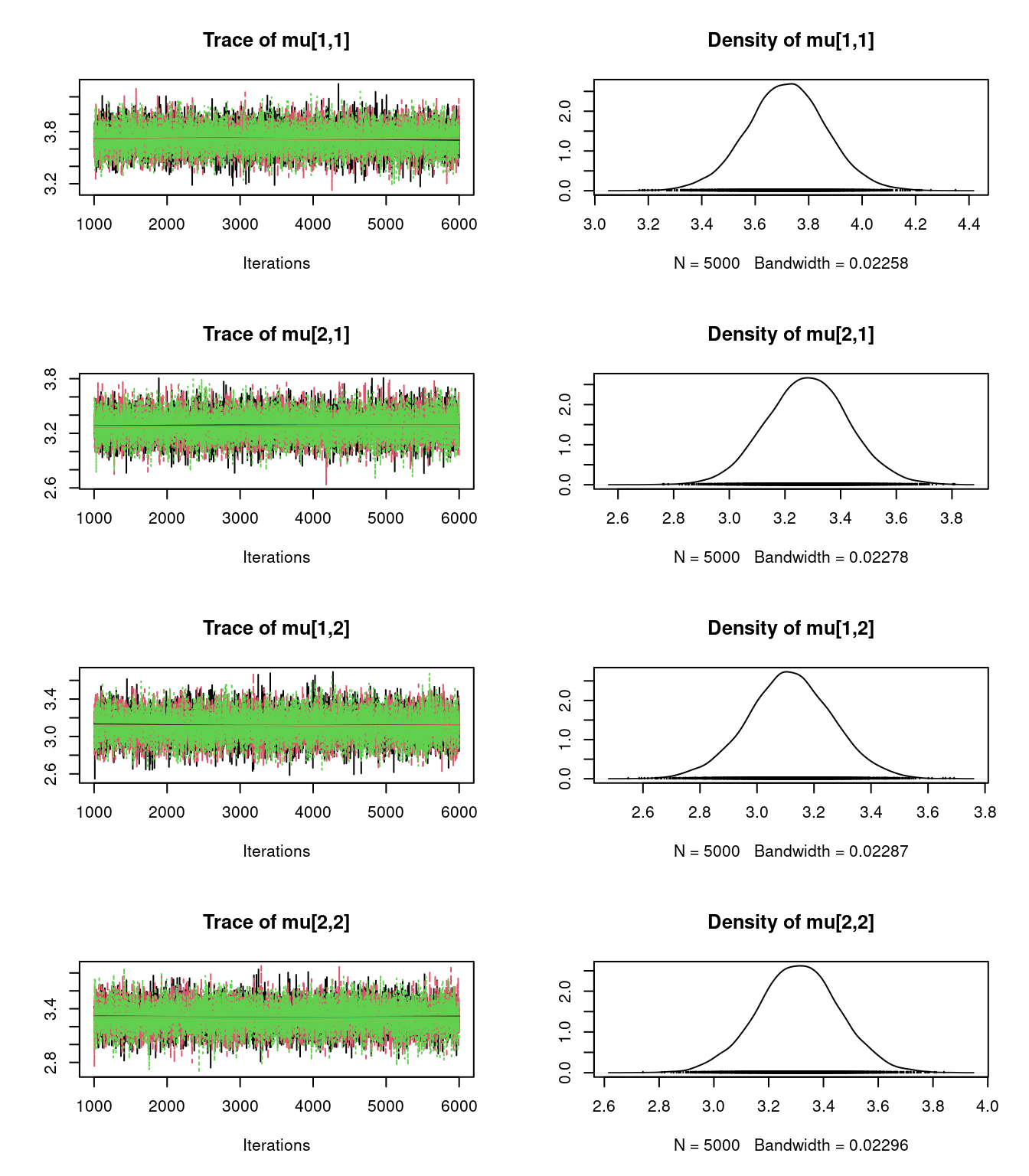
## convergence diagnostics
gelman.diag(mod3_sim)
Potential scale reduction factors:
Point est. Upper C.I.
mu[1,1] 1 1
mu[2,1] 1 1
mu[1,2] 1 1
mu[2,2] 1 1
mu[1,3] 1 1
mu[2,3] 1 1
sig 1 1
Multivariate psrf
1autocorr.diag(mod3_sim) mu[1,1] mu[2,1] mu[1,2] mu[2,2] mu[1,3]
Lag 0 1.000000000 1.0000000000 1.000000000 1.000000000 1.000000000
Lag 1 -0.003950451 -0.0115467646 0.000151158 0.005399061 0.001249259
Lag 5 -0.002132338 -0.0202316439 -0.001697396 -0.005183778 -0.003977682
Lag 10 0.003945287 -0.0058879242 0.002867066 0.005943263 0.010477095
Lag 50 0.022810358 0.0004434449 0.007473512 0.007570026 -0.007551555
mu[2,3] sig
Lag 0 1.000000000 1.000000000
Lag 1 0.008328452 0.095924507
Lag 5 0.002049641 0.003040122
Lag 10 0.005985258 0.010193322
Lag 50 0.007968976 -0.005965982effectiveSize(mod3_sim) mu[1,1] mu[2,1] mu[1,2] mu[2,2] mu[1,3] mu[2,3] sig
14907.91 15000.00 14698.45 14791.66 14570.75 14795.57 11505.00 raftery.diag(mod3_sim)[[1]]
Quantile (q) = 0.025
Accuracy (r) = +/- 0.005
Probability (s) = 0.95
Burn-in Total Lower bound Dependence
(M) (N) (Nmin) factor (I)
mu[1,1] 2 3803 3746 1.020
mu[2,1] 2 3803 3746 1.020
mu[1,2] 2 3803 3746 1.020
mu[2,2] 2 3930 3746 1.050
mu[1,3] 2 3866 3746 1.030
mu[2,3] 2 3620 3746 0.966
sig 2 3741 3746 0.999
[[2]]
Quantile (q) = 0.025
Accuracy (r) = +/- 0.005
Probability (s) = 0.95
Burn-in Total Lower bound Dependence
(M) (N) (Nmin) factor (I)
mu[1,1] 2 3680 3746 0.982
mu[2,1] 2 3866 3746 1.030
mu[1,2] 2 3620 3746 0.966
mu[2,2] 2 3680 3746 0.982
mu[1,3] 2 3680 3746 0.982
mu[2,3] 2 3995 3746 1.070
sig 2 3680 3746 0.982
[[3]]
Quantile (q) = 0.025
Accuracy (r) = +/- 0.005
Probability (s) = 0.95
Burn-in Total Lower bound Dependence
(M) (N) (Nmin) factor (I)
mu[1,1] 2 3866 3746 1.030
mu[2,1] 2 3741 3746 0.999
mu[1,2] 2 3680 3746 0.982
mu[2,2] 2 3866 3746 1.030
mu[1,3] 2 3620 3746 0.966
mu[2,3] 2 3741 3746 0.999
sig 2 3866 3746 1.030 Let’s compute the DIC and compare with our previous models.
(dic3 = dic.samples(mod3, n.iter=1e3))Mean deviance: 52.04
penalty 7.229
Penalized deviance: 59.27 dic2Mean deviance: 55.51
penalty 5.074
Penalized deviance: 60.58 dic1Mean deviance: 66.47
penalty 4.026
Penalized deviance: 70.5 This suggests that the full model with interaction between wool and tension (which is equivalent to the cell means model) is the best for explaining/predicting warp breaks.
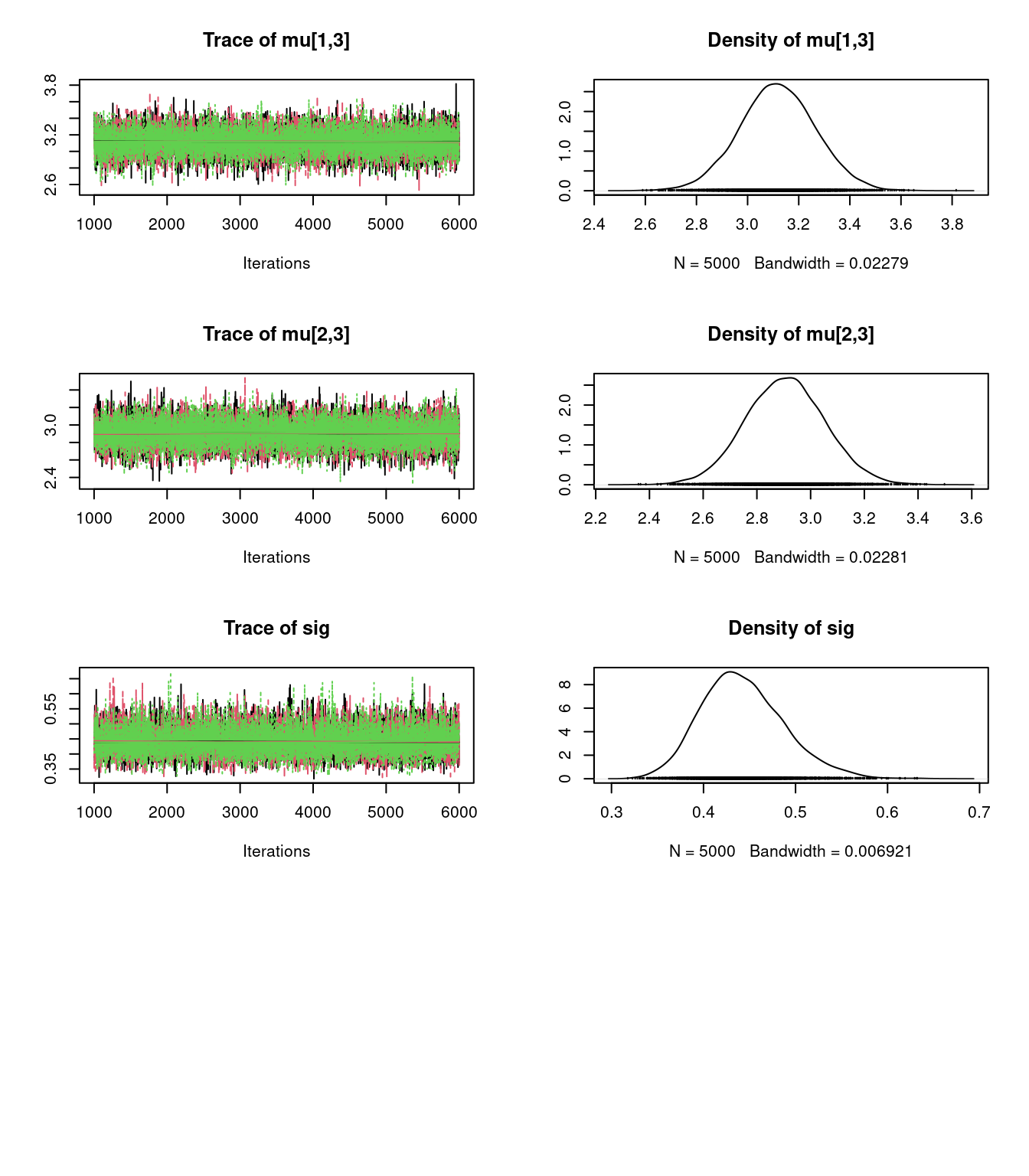
summary(mod3_sim)
Iterations = 1001:6000
Thinning interval = 1
Number of chains = 3
Sample size per chain = 5000

1. Empirical mean and standard deviation for each variable,
   plus standard error of the mean:

          Mean      SD Naive SE Time-series SE
mu[1,1] 3.7179 0.14844 0.001212      0.0012157
mu[2,1] 3.2792 0.14792 0.001208      0.0012078
mu[1,2] 3.1168 0.14869 0.001214      0.0012270
mu[2,2] 3.3082 0.14963 0.001222      0.0012304
mu[1,3] 3.1187 0.14865 0.001214      0.0012352
mu[2,3] 2.9046 0.14757 0.001205      0.0012134
sig     0.4434 0.04495 0.000367      0.0004205

2. Quantiles for each variable:

          2.5%    25%    50%    75%  97.5%
mu[1,1] 3.4223 3.6195 3.7195 3.8169 4.0053
mu[2,1] 2.9882 3.1812 3.2811 3.3768 3.5695
mu[1,2] 2.8277 3.0179 3.1146 3.2150 3.4158
mu[2,2] 3.0149 3.2076 3.3071 3.4074 3.6051
mu[1,3] 2.8290 3.0182 3.1169 3.2182 3.4146
mu[2,3] 2.6157 2.8043 2.9046 3.0032 3.1961
sig 0.3662 0.4121 0.4401 0.4707 0.5404HPDinterval(mod3_csim) lower upper
mu[1,1] 3.4342328 4.0153071
mu[2,1] 2.9980428 3.5773164
mu[1,2] 2.8292920 3.4167252
mu[2,2] 3.0245498 3.6138570
mu[1,3] 2.8373407 3.4210593
mu[2,3] 2.6094649 3.1873873
sig 0.3623452 0.5341155
attr(,"Probability")
[1] 0.95par(mfrow=c(3,2)) # arrange frame for plots
densplot(mod3_csim[,1:6], xlim=c(2.0, 4.5))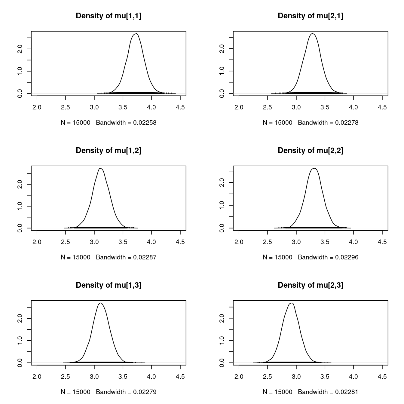
It might be tempting to look at comparisons between each combination of treatments, but we warn that this could yield spurious results. When we discussed the statistical modeling cycle, we said it is best not to search your results for interesting hypotheses, because if there are many hypotheses, some will appear to show “effects” or “associations” simply due to chance. Results are most reliable when we determine a relatively small number of hypotheses we are interested in beforehand, collect the data, and statistically evaluate the evidence for them.
One question we might be interested in with these data is finding the treatment combination that produces the fewest breaks. To calculate this, we can go through our posterior samples and for each sample, find out which group has the smallest mean. These counts help us determine the posterior probability that each of the treatment groups has the smallest mean.
prop.table( table( apply(mod3_csim[,1:6], 1, which.min) ) )
         2          3          4          5          6
0.01633333 0.12286667 0.00920000 0.11326667 0.73833333
The evidence supports wool B with high tension as the treatment that produces the fewest breaks.