# Generate n observations from a mixture of two Gaussian distributions
n     = 50           # required sample size
w     = c(0.6, 0.4)  # mixture weights
mu    = c(0, 5)      # list of means
sigma = c(1, 2)      # list of sds
cc    = sample(1:2, n, replace=T, prob=w) # sample for the component selector
x = rnorm(n, mu[cc], sigma[cc]) # sample the selected component60.1 Hierarchical representations 🎥
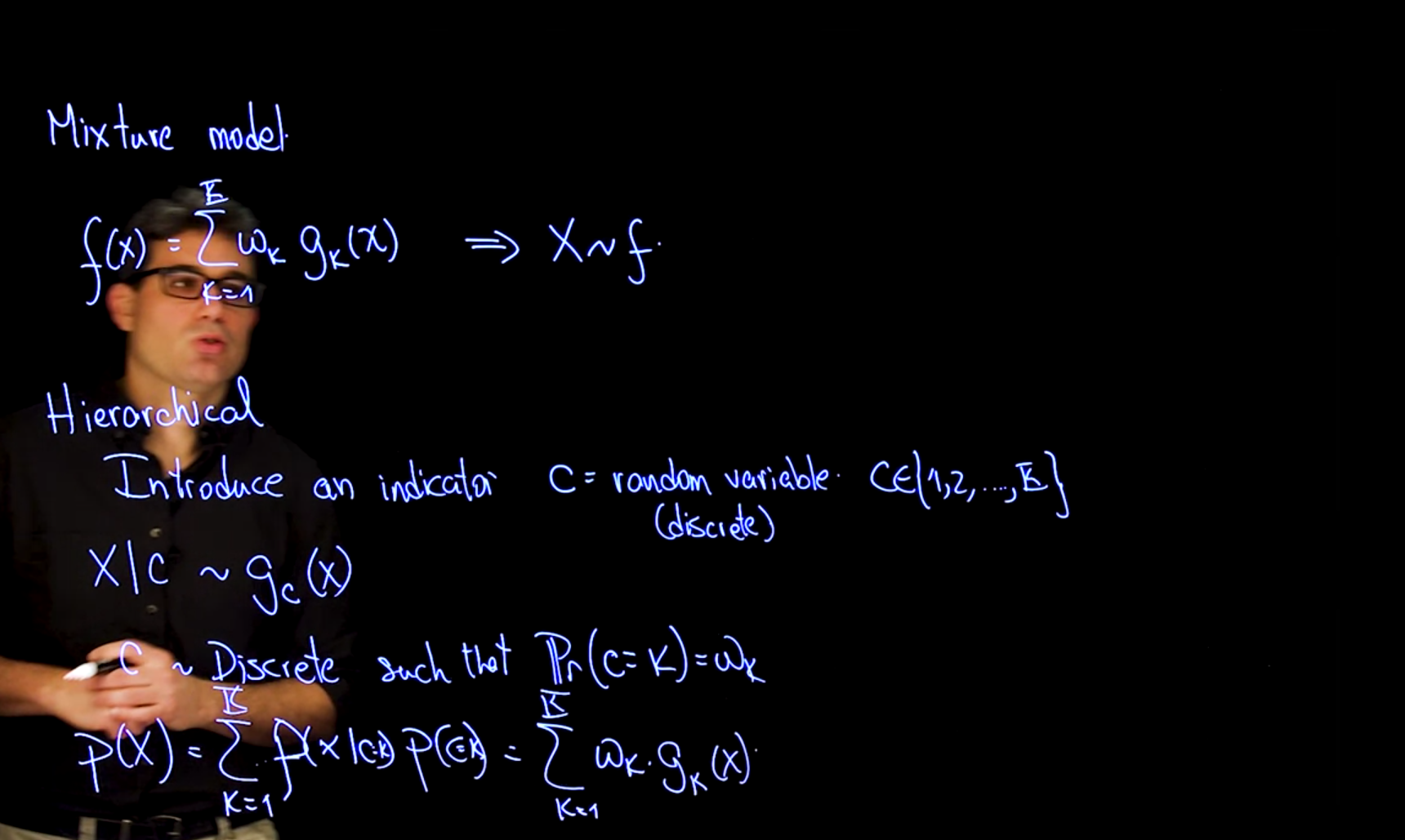
Recall that the cumulative distribution function of a mixture takes the form Equation 55.1, where G_k(x) is the cumulative distribution function of the k-th component of the mixture.
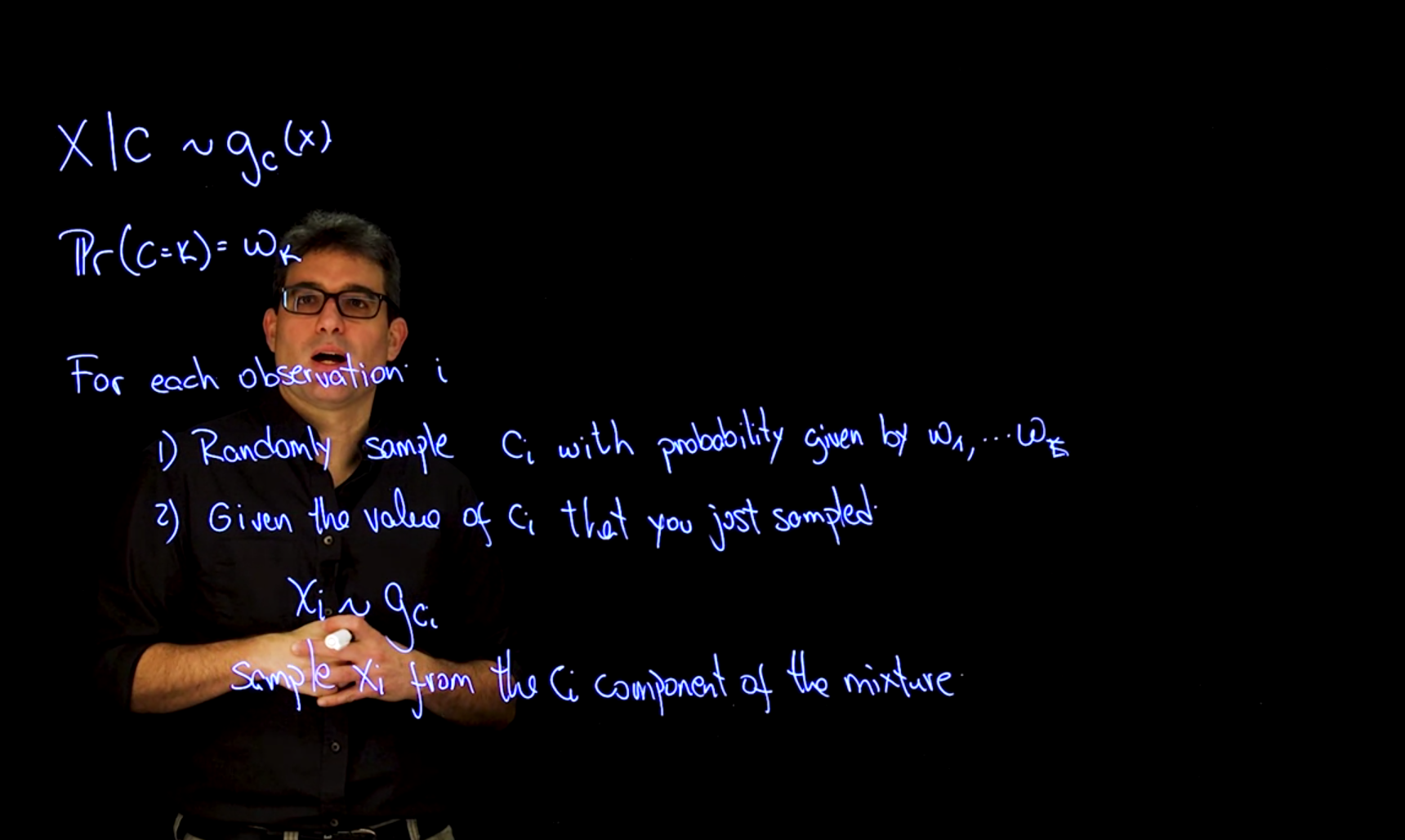
We can use a RV for each component and introduce an indicator RV for the component selector C_i to select the component from which we will sample. This results in a hierarchical representation of the mixture model.
X \mid c \sim g_c(x) \qquad \mathbb{P}r(c=k) = \omega_k \qquad \tag{60.1}
where C is a categorical random variable with K categories, and G_k(x \mid C=k) is the cumulative distribution function of the k-th component of the mixture given that we have selected the k-th component.
This allows us to write the cumulative distribution function of the mixture as a weighted sum of the cumulative distribution functions of the components
\begin{aligned} \mathbb{P}r(x) &= \sum^K_{k=1} \mathbb{P}r(x \mid C=k) \cdot \mathbb{P}r(C=k) \\ &= \sum^K_{k=1} g_k(x) \cdot \omega_k \qquad \end{aligned} \tag{60.2}
- where
- g_k(x) is the cumulative distribution function of the kth component of the mixture.
- \omega_k is the weight of the kth component of the mixture, and
- C is a categorical random variable with K categories, and \mathbb{P}r(C=k) = \omega_k is the probability of selecting the kth component of the mixture.
60.2 Code for simulating from a Mixture Model 📓 \mathcal{R} 🐍
# Plot f(x) along with the observations just sampled
xx = seq(-5, 12, length=200)
yy = w[1] * dnorm(xx, mu[1], sigma[1]) + w[2] * dnorm(xx, mu[2], sigma[2])
par(mar=c(4,4,1,1)+0.1)
plot(xx, yy, type="l", ylab="Density", xlab="x", las=1, lwd=2)
points(x, y=rep(0,n), pch=1, col=cc)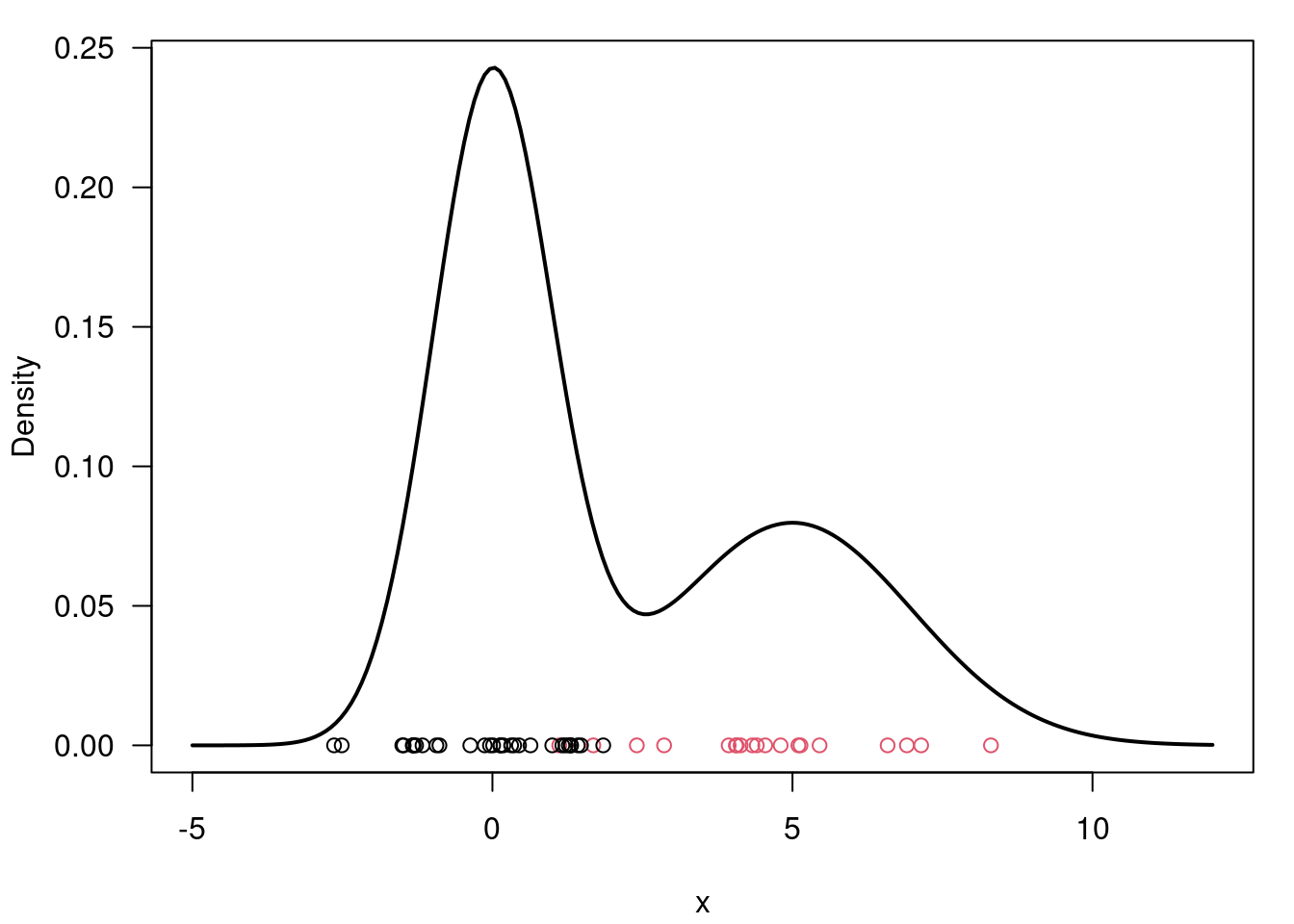
import numpy as np
import matplotlib.pyplot as plt
import scipy.stats as stats
from scipy.stats import norm

n=50           # required sample size
w=[0.6, 0.4]  # mixture weights
mu=[0, 5]      # list of means
sigma=[1, 2]  # list of sds
cc = np.random.choice([0, 1], size=n, p=w) # sample for the component selector
# sample the selected component
x = np.array([np.random.normal(mu[i], sigma[i]) for i in cc])
# Plot f(x) along with the observations just sampled
xx = np.linspace(-5, 12, num=200)
yy = w[0]*norm.pdf(loc=mu[0], scale=sigma[0], x=xx) + \
w[1]*norm.pdf(loc=mu[1], scale=sigma[1], x=xx)
plt.plot(xx, yy, label='Mixture of Gaussians')
plt.scatter(x, np.zeros(n), c=cc, label='Sampled data')
plt.xlabel('x')
plt.ylabel('Density')
plt.title('Mixture of Gaussians')
plt.legend()
plt.show() 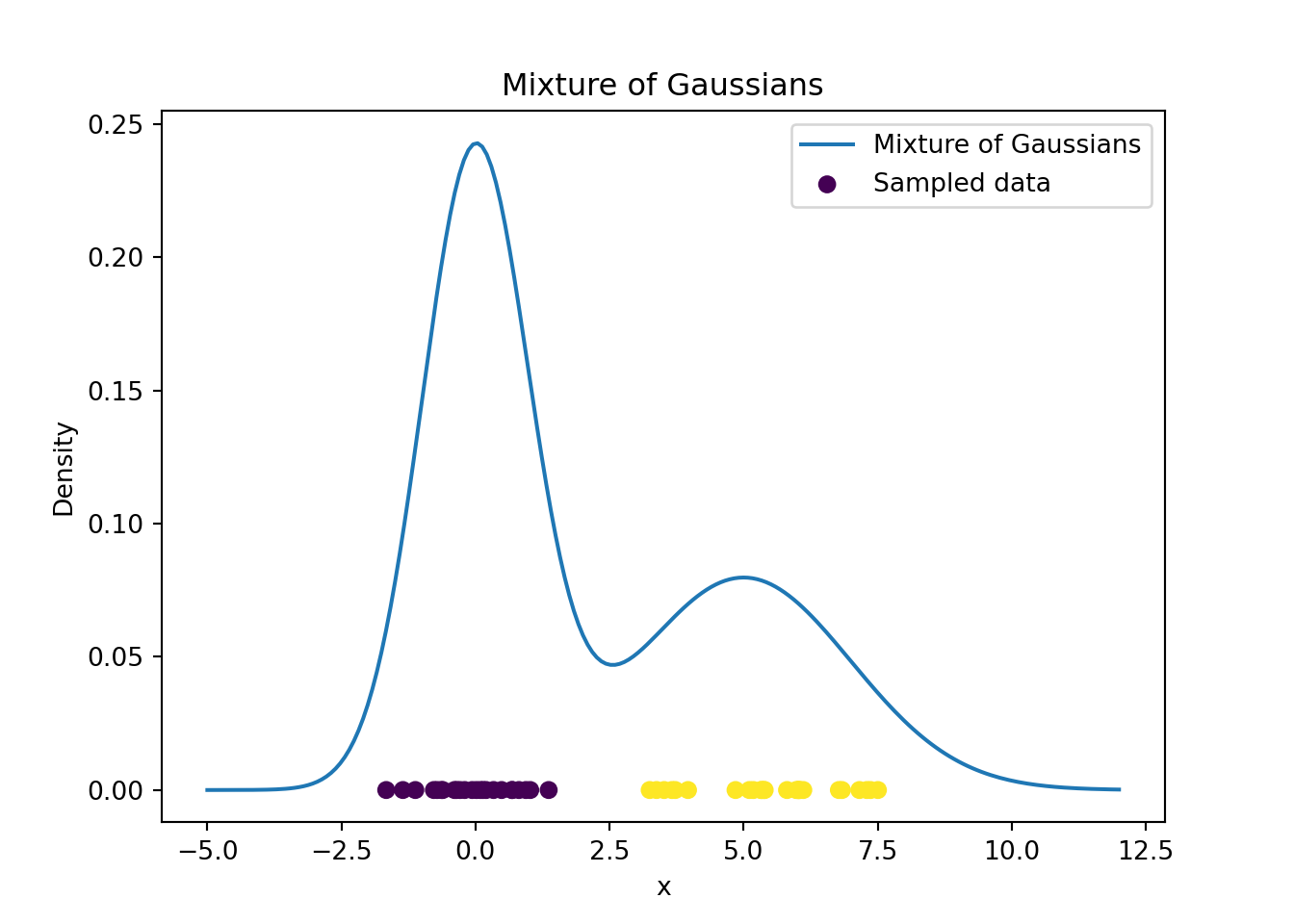
60.3 The Likelihood function 🎥
ImportantLikelihood functions for Mixture Models
We will use the complete data likelihood extensively in this and the upcoming two courses. So I’ve made added the annotation and interpretation to the math. The almost ubiquitous use of the complete data likelihood is one of the main reasons why we use the hierarchical representation of the mixture model and is worth extra attention if you wish to fully comprehend the upcoming model of the specialization.
We are now moving on to inferring the parameters of the mixture model from the observed data.
We can estimate these using the maximum likelihood estimation or with Bayesian estimation.
In both cases we will need to compute the likelihood of the observed data.
We can construct two different types of likelihood function:
- the observed data likelihood, which just uses the original representation of the mixture model as a weighted sum, is the probability of observing the data given the parameters of the model.
- the complete data likelihood is the probability of observing the data and the latent variables given the parameters of the model. This is called the complete data likelihood, and it relies on the hierarchical representation from Section 60.1.
60.3.1 Observed data likelihood
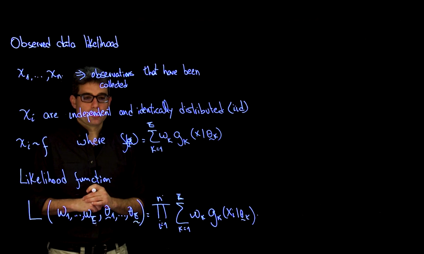
Our assumption is that we have a set of observations \mathbf{x} = (x_1, \ldots, x_n), which are independent and identically distributed (i.i.d.) samples from the mixture distribution.
We model them using a mixture, such as we have seen in Equation 60.2.
\mathbf{x}_i \sim f \qquad f(\mathbf{x} ) = \sum_{k=1}^K w_k \cdot g_k(x_i \mid \boldsymbol{\theta_k}) \tag{60.3}
- where:
- \omega_k is the weights of the kth mixture components,
- g_k(x_i \mid \theta) is the probability density function of the kth mixture component, and
- \boldsymbol{\theta} are the parameters of the components.
The likelihood function is proportional to the joint distribution so we can construct it by taking the product of the probability density functions of the individual components, weighted by their respective weights which gives us the observed data likelihood. Note that this is possible because we have assumed that the observations are independent and identically distributed (i.i.d.).1
The observed data likelihood is the probability of observing the data given the parameters of the model
\mathcal{L}(\boldsymbol{\omega},\boldsymbol{\theta} \mid \mathbf{x}) = \prod_{i=1}^n \sum_{k=1}^K w_k \cdot g_k(x_i \mid \theta_k) \tag{60.4}
- where
- g_k(x_i \mid \theta) is the probability density function of the k-th component of the mixture, with
- \boldsymbol{\omega} are the weights of the mixture components.
- \boldsymbol{\theta_k} are the parameters of the components.
We call this the observed data likelihood because we have already observed the data and so the parameters for this likelihood are the weights and the parameters of the components.
CautionWhy we don’t use the observed data likelihood?
Unfortunately, the observed data likelihood is not easy to work with because it involves a sum over the components of the mixture. This is why we often use the complete data likelihood which is easier to work with.
60.3.2 Complete data likelihood
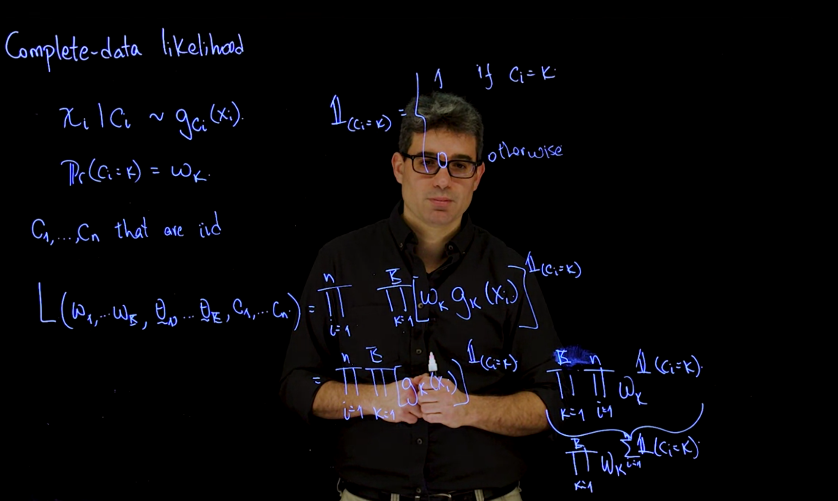
we now introduce the latent variable C_i which indicates which component generated the observation x_i. x_i \mid C_i \sim g_{C_i}(x_i \mid \theta_{C_i}) \qquad \mathbb{P}r(C_i=k) = w_k \qquad C_i \stackrel{i.i.d.}{\sim} \text{Categorical}(\boldsymbol{\omega})
we can now introduce an indicator variable based on C_i that indicates which component generated the observation x_i.
\mathbb{I}_{(C_i=k)} = \begin{cases} 1 & \text{if } C_i=k \\ 0 & \text{otherwise} \end{cases} \tag{60.5}
This reparametrization allows expressing the joint likelihood compactly over all possible latent assignments.
\begin{aligned} \mathcal{L}(\boldsymbol{\omega},\boldsymbol{\theta}, \mathbf{C}) &= \prod_{i=1}^n \prod_{k=1}^K [\omega_k g_k(x_i)]^{\mathbb{I}_{(C_i=k)}} \\ &= \prod_{i=1}^n \prod_{k=1}^K [ g_k(x_i) ]^{\mathbb{I}_{(C_i=k)}} \cdot \prod_{i=1}^n \prod_{k=1}^K \omega_k ^{\mathbb{I}_{(C_i=k)}} \\ &= \underbrace{ \prod_{i=1}^n \prod_{k=1}^K [ g_k(x_i) ]^{\mathbb{I}_{(C_i=k)}} }_{\text{conditional likelihood}} \cdot \underbrace{ \prod_{k=1}^K \omega_k ^{ \overbrace{\sum_{i=1}^n \mathbb{I}_{(C_i=k)} }^{\text{no. observations in } C_k }} }_{\text{marginal likelihood of } C_k } \end{aligned} \tag{60.6}
- The left hand term corresponds to the conditional likelihood: p(x_i \mid C_i, \theta_{C_i}).
- The right hand term is the marginal likelihood of the latent variables: p(C_i \mid \boldsymbol{\omega}).
How did we get the sum in the exponent of the second term?
In the last step it is possible to replace one of the product on the right hand side with a sum inside the power because the basis of this expression is the same i.e. \omega_i for every i. And an exponent is just a shorthand for product with the same base.
What does the the sum represents?
We can see it’s just the number of observations in the sample that belong to up to component k.
How can we interpret this form of the likelihood function?
That provides a very nice break, and a very nice interpretation for the likelihood function, and for a complete data likelihood function. We have one piece of the likelihood function that corresponds to the distribution of the observations.
Basically, if we know what component generated each observation, we use the density of that component in this product, which simplifies this expression substantially.
We are going to retain for each i one of the key terms that corresponds to the exponent that is equal to one. Then, we have a second term that corresponds to this product of the weights. In every case, the weight is going to be raised to essentially the number of observations, that belong to that component.
This allows us to write the complete data likelihood as a product of the likelihoods of the individual components, weighted by their respective weights. This formulation is conjugate-friendly and facilitates both Gibbs sampling and the E-step in the EM algorithm
60.4 Parameter identifiability 🎥
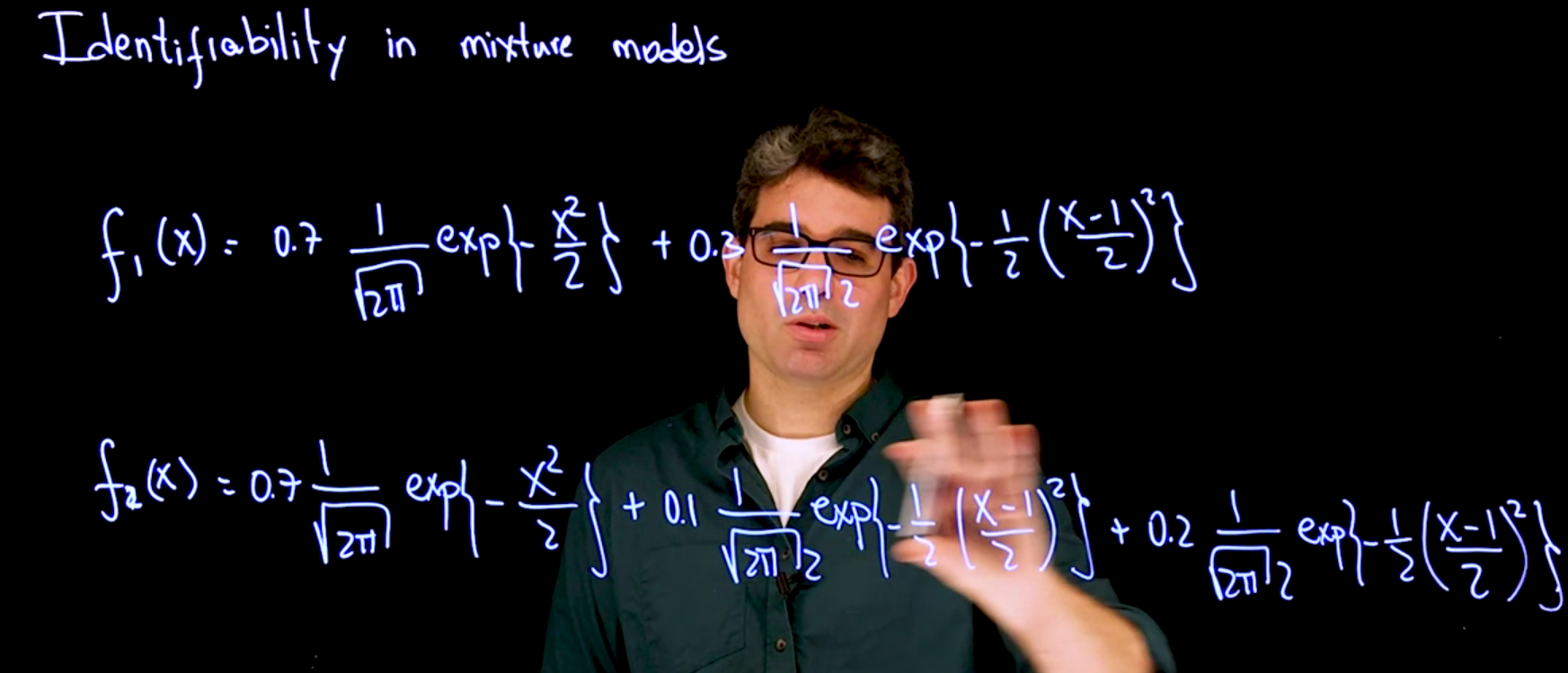
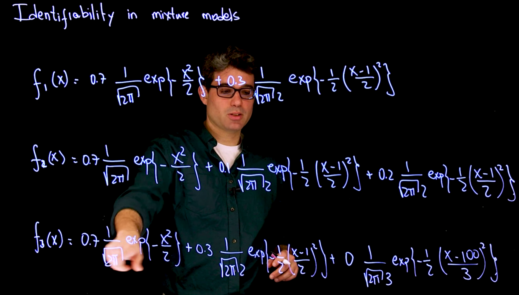
A probability model is identifiable if and only if different values of the parameters generate different probability distributions of the observable variables.
One challenge involved in working with mixture models is that they are not fully identifiable.
The problem is that different representations exists for the same mixture.
Question: Is there a “Canonical representation” which fixes this, essentially a convention like:
1. picking the representation with the least components (no zero weights)
2. ordered with descending w_i
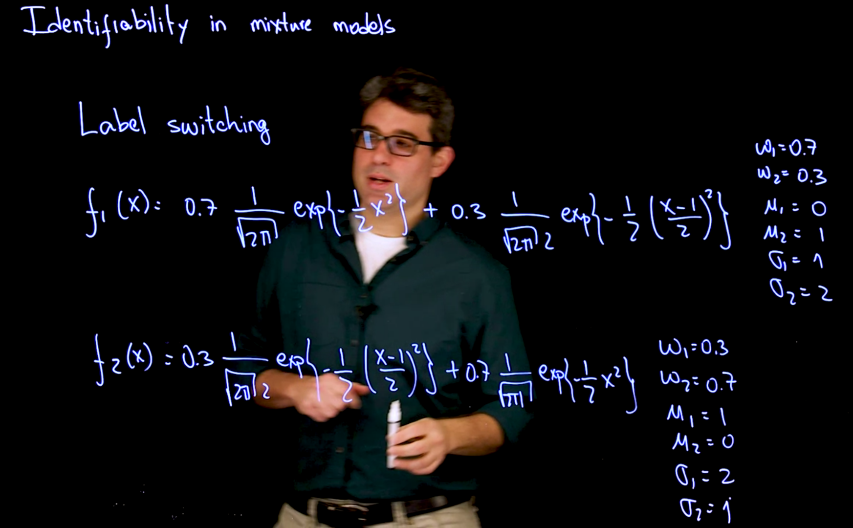
60.4.1 Label switching
The labels used to distinguish the components in the mixture are not identifiable. The literature sometimes refers to this type of lack of identifiability as the label switching “problem”. Whether label switching is an actual problem or not depends on the computational algorithm being used to fit the model, and the task we are attempting to complete in any particular case. For example, label switching tends to not be an issue for the purpose of density estimation or classification problems, but it can lead to serious difficulties in clustering problems.
de Finetti’s theorem might allow us to make this step using a weaker assumption on the exchangeability of the observations.↩︎