lg = function(mu, n, ybar) {
  mu2 = mu^2
  n * (ybar * mu - mu2 / 2.0) - log(1 + mu2)
}
NoteLearning Objectives
- Understand the basics of MCMC including Metropolis-Hastings and Gibbs sampling.
- Write a statistical model in JAGS and produce posterior samples by calling JAGS from R.
- Assess MCMC output to determine if it is suitable for inference.
33.1 Markov chain Monte Carlo (MCMC)
Metropolis-Hastings (M-H) is an algorithm that allows us to sample from a generic probability distribution (which we will call the target distribution), even if we do not know the normalizing constant. To do this, we construct and sample from a Markov chain whose stationary distribution is the target distribution. It consists of picking an arbitrary starting value and iteratively accepting or rejecting candidate samples drawn from another distribution, one that is easy to sample.
ImportantWhy use M-H or MCMC?
We will use M-H or other MCMC methods if there is no easy way to simulate independent draws from the target distribution. This can be due to non-conjugate priors, challenges in evaluating the normalizing constant or multiple explanatory variables.
33.2 The Metropolis-Hastings Algorithm 🎥
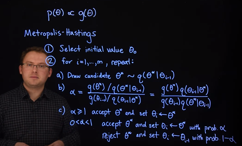
Let’s say we wish to produce samples from a target distribution \mathbb{P}r(\theta) \propto g(\theta), where we don’t know the normalizing constant (since \int g(\theta)d\theta is hard or impossible to compute), so we only have g(\theta), the unnormalized joint probability to work with. The Metropolis-Hastings algorithm proceeds as follows.
- Select an initial value \theta_0.
- For i=1,\dots,m repeat the following steps:
- Draw a candidate sample \theta^∗ from a proposal distribution q(\theta^* \mid \theta_{i−1}) .
- Compute the ratio \alpha = \frac{g(\theta^*) / q(\theta^* \mid \theta_{i-1}) }{g(\theta_{i-1}) / q(\theta_{i-1} \mid \theta^*)} = \frac{g(\theta^*)q(\theta_{i-1} \mid \theta^*)}{g(\theta_{i-1})q(\theta^* \mid \theta_{i-1})}
- If \alpha\ge 1, then accept \theta^∗ and set \theta_i=\theta^∗.
- If 0<\alpha<1:
- accept \theta^∗ and set \theta_i=\theta^∗ with probability \alpha,
- reject \theta^∗ and set \theta_i=\theta_{i−1} with probability 1−\alpha.
proposal distribution q
ImportantCorrection to the proposal distribution
Steps 2.b and 2.c act as a correction since the proposal distribution is not the target distribution. At each step in the chain, we draw a random candidate value of the parameter and decide whether to “move” the chain there or remain where we are. If the proposed move to the candidate is “advantageous,” (\alpha \ge 1) we “move” there and if it is not “advantageous,” we still might move there, but only with probability \alpha. Since our decision to “move” to the candidate only depends on where the chain currently is, this is a Markov chain.
correction
33.3 Proposal distribution q
One careful choice we must make is the candidate generating distribution q(\theta^∗\mid\theta_{i−1}). It may or may not depend on the previous iteration’s value of \theta.
ImportantIndependent Metropolis-Hastings
The simpler case is when the proposal distribution q does not depend on the previous value. We then write it as q(\theta^∗). This arises if it is always the same distribution. We call this case independent Metropolis-Hastings. If we use independent M-H, q(\theta) should be as similar as possible to \mathbb{P}r(\theta).
ImportantRandom-Walk Metropolis-Hastings
In the more general case, the proposal distribution takes the form q(\theta^∗\mid\theta_{i−1}) with dependence on the previous iteration, is Random-Walk Metropolis-Hastings. Here, the proposal distribution is centered on \theta_{i−1}.
For instance, it might be a Normal distribution with mean \theta_{i−1}. Because the Normal distribution is symmetric, this example comes with another advantage: q(\theta^* \mid \theta_{i−1})=q(\theta_{i−1}∣\theta^*) causing it to cancel out when we calculate \alpha.
Thus, in Random-Walk M-H where the candidate is drawn from a Normal with mean \theta_{i−1} and constant variance, the acceptance ratio is simply \alpha=g(\theta^∗)/g(\theta_{i−1}).
33.4 Acceptance rate \alpha
Clearly, not all candidate draws are accepted, so our Markov chain sometimes “stays” where it is, possibly for many iterations. How often you want the chain to accept candidates depends on the type of algorithm you use. If you approximate \mathbb{P}r(\theta) with q(\theta^∗) and always draw candidates from that, accepting candidates often is good; it means q(\theta^∗) is approximating \mathbb{P}r(\theta) well. However, you still may want q to have a larger variance than p and see some rejection of candidates as an assurance that q is covering the space well.
As we will see in coming examples, a high acceptance rate for the Random-Walk Metropolis-Hastings sampler is not a good thing. If the random walk is taking too small of steps, it will accept often but will take a very long time to fully explore the posterior. If the random walk is taking too large of steps, many of its proposals will have a low probability and the acceptance rate will be low, wasting many draws. Ideally, a random walk sampler should accept somewhere between 23% and 50% of the candidates proposed.
In the next segment, we will see a demonstration of this algorithm used in a discrete case, where we can show mathematically that the Markov chain converges to the target distribution. In the following segment, we will demonstrate coding a Random-Walk Metropolis-Hastings algorithm in R to solve one of the problems from the end of Lesson 2.
33.5 Demonstration of a Discrete case
The following segment is by Herbert Lee, a professor of statistics and applied mathematics at the University of California, Santa Cruz.
The following is a demonstration of using Markov chain Monte Carlo, used to estimate posterior probabilities in a simplified case, where we can actually work out the correct answer in closed form. We demonstrate that the Metropolis-Hastings algorithm is indeed working, and giving us the right answer.
If you recall from the previous course, the example where your brother or maybe your sister, has a loaded coin that you know will come up heads 70% of the time. But they come to you with some coin, you’re not sure if it’s the loaded coin or a fair coin, and they want to make a bet with you. And you have to figure out which coin this is.
Suppose you have a prior probability that it’s a 60% probability, that they’ll bring a loaded coin to you. They let you flip it five times, and you get two heads and three tails.
And then you need to figure out, what’s your posterior probability that this is a loaded coin.
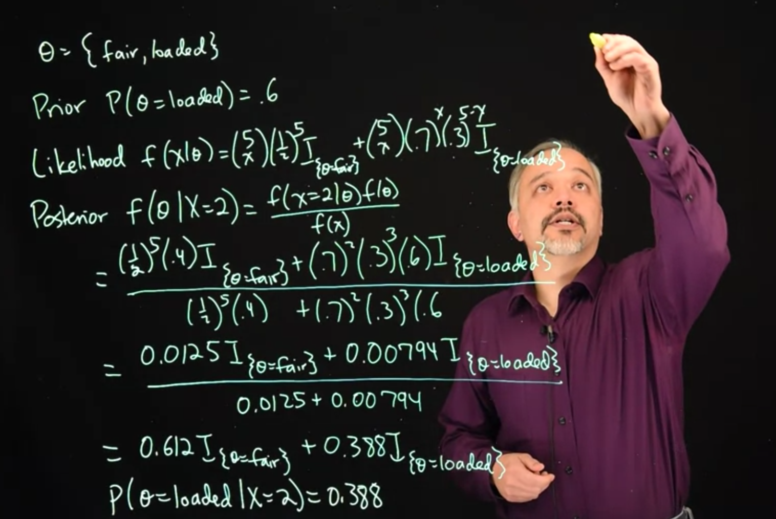
Our unknown parameter \theta, can either take the values fair or loaded.
\theta = \{\text{fair, loaded} \} \tag{33.1}
Our prior for \theta is the probability of theta equals loaded, is 0.6.
\mathbb{P}r(\theta=\text{loaded})=0.6 \qquad \text{(prior)} \tag{33.2}
Our likelihood will follow a Binomial distribution, depending upon the value of \theta.
f(x\mid \theta) = {5 \choose x} \frac{1}{2}^5\mathbb{I}_{\theta=\text{fair}}+ {5 \choose x} (.7)^x(.3)^{5-x}\mathbb{I}_{\theta=\text{loaded}} \qquad \text{(likelihood)} \tag{33.3}
Our posterior then, we can look at posterior for theta, given that we saw x=2 equals two heads, posterior is the likelihood times the prior, divided by a normalizing constant.
\begin{aligned} f(\theta \mid X=2) &= \frac{ \frac{1}{2}^5(0.4)\mathbb{I}_{(\theta=\text{fair})} + (.7)^2(.3)^{3}(.6)\mathbb{I}_{(\theta=\text{loaded})}} { \frac{1}{2}^5(0.4) + (.7)^2(.3)^{3}(.6)} \\&=\frac{ 0.0125 \mathbb{I}_{(\theta=\text{fair})} + 0.00794 \mathbb{I}_{(\theta=\text{loaded})}} { 0.0125 + 0.00794} \\&= 0.612 \mathbb{I}_{(\theta=\text{fair})} + 0.388 \mathbb{I}_{(\theta=\text{loaded})} \qquad \text{(posterior) } \end{aligned} \tag{33.4}
In this case, we can work out the binomial and our prior. And we see that we get these expressions at the end. We get posterior probability of \theta is loaded given that we saw two heads, to be 0.388.
\therefore \mathbb{P}r(\theta=\text{loaded}\mid X=2) = 0.388 \qquad \text{(posterior conditional probability ) } \tag{33.5}
This is all review from the previous course so far.
But suppose we had a more complicated problem, where we couldn’t work this all out in closed form? We’ll know the likelihood and the prior, but we may not be able to get this normalizing constant. Can we instead do this by simulation? And indeed, yes we can.
We can do this with Markov chain Monte Carlo. In particular, using the Metropolis-Hastings algorithm. What we’ll do is, we’ll set up a Markov chain whose equilibrium distribution has this posterior distribution. So we’ll consider a Markov chain with two states, theta equals fair and theta equals loaded. And we’ll allow the chain to move between those two states, with certain transition probabilities. We set this up using this using the Metropolis-Hastings algorithm.
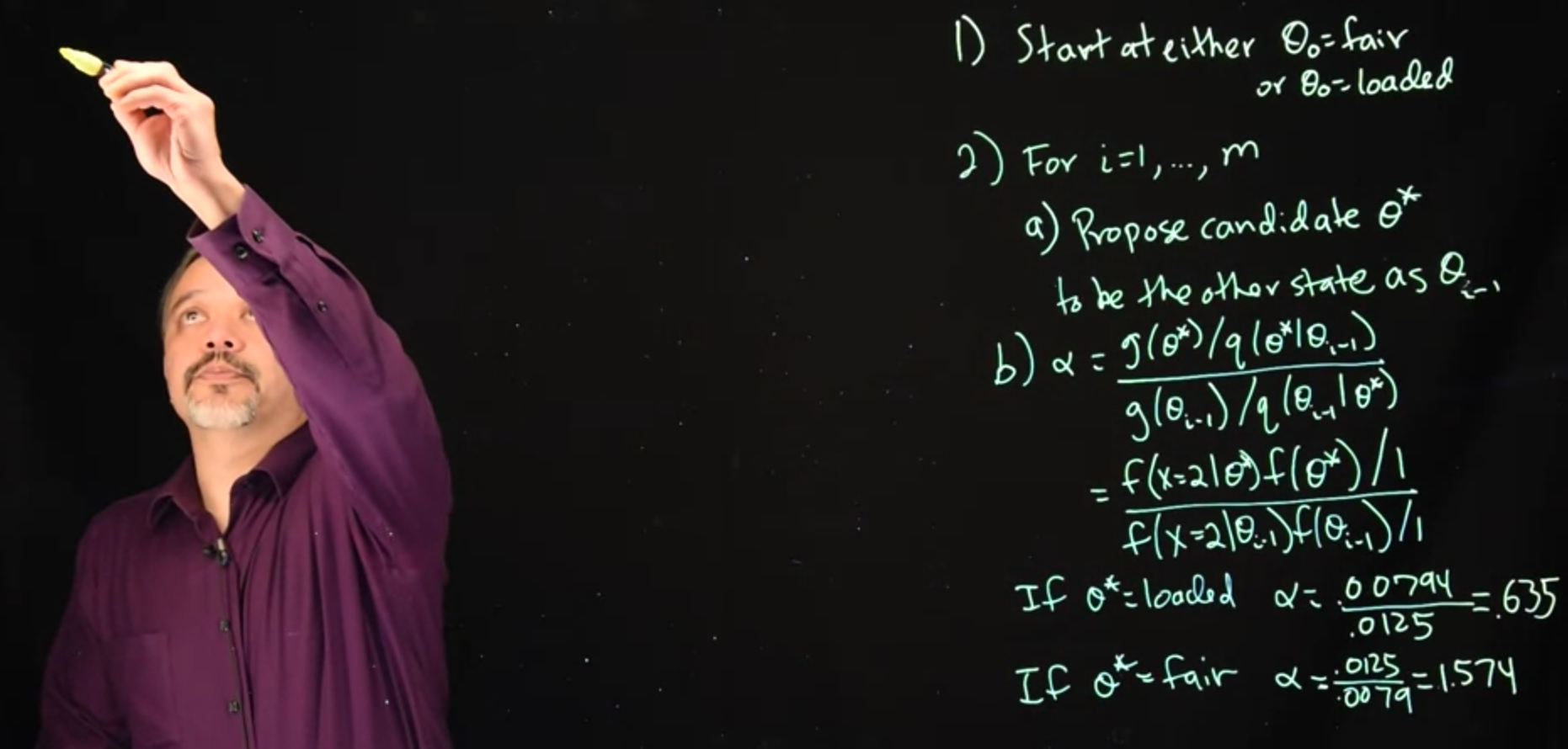
So under the Metropolis-Hastings algorithm, step one is we start at an arbitrary location. And in this case, we can
- start at either \theta \ne \text{fair}, or \theta \ne \text{loaded}.
It does not really matter where we start, we’ll be moving back and forth and we’re going to look at the long-term running average, the long-term simulations.
So the key is we’ll be simulating.
- Run m simulations and in each iteration, we’ll propose a candidate and either accept it or reject it.
- So the first part is we’re proposing a new candidate. We’ll call this candidate \theta^*, and we’re going to propose it be the other state compared to where we are now. Where we are now is \theta_{i-1}, and so we’ll propose to move to \theta^*.
- If our current state is
fair, we’ll propose \theta^*=\text{loaded}. - If our current state is
loaded, we’ll propose \theta^*=\text{fair}.
- If our current state is
what’s our acceptance probability alpha?
The general form for \alpha is:
\begin {aligned} \alpha &= { { g(\theta^*) / q(\theta^* \mid \theta_{i-1}) } \over {g(\theta_{i-1}) / q(\theta_{i-1} \mid \theta^*) } }\\ &= { { f(x=2 \mid \theta^*) f(\theta^*) / 1 } \over { f(x=2 \mid \theta_{i-1})f(\theta_{i-1}) / 1 } } \qquad \text {(sub. g,q)} \end{aligned} \tag{33.6}
In this case,
- g() is our un-normalized likelihood times prior
- q(), the proposal distribution, is, in this case, since we always accept the opposite state deterministically i.e. \theta^*=\neg \theta{i_1} with P=1
- If \theta^* = \text{loaded} \implies \alpha = {0.00794 \over 0.0125}=0.635
- If \theta^* = \text{fair} \implies \alpha = { 0.0125 \over 0.00794}=1.574
Given these probabilities, we then can do the acceptance or rejection step.
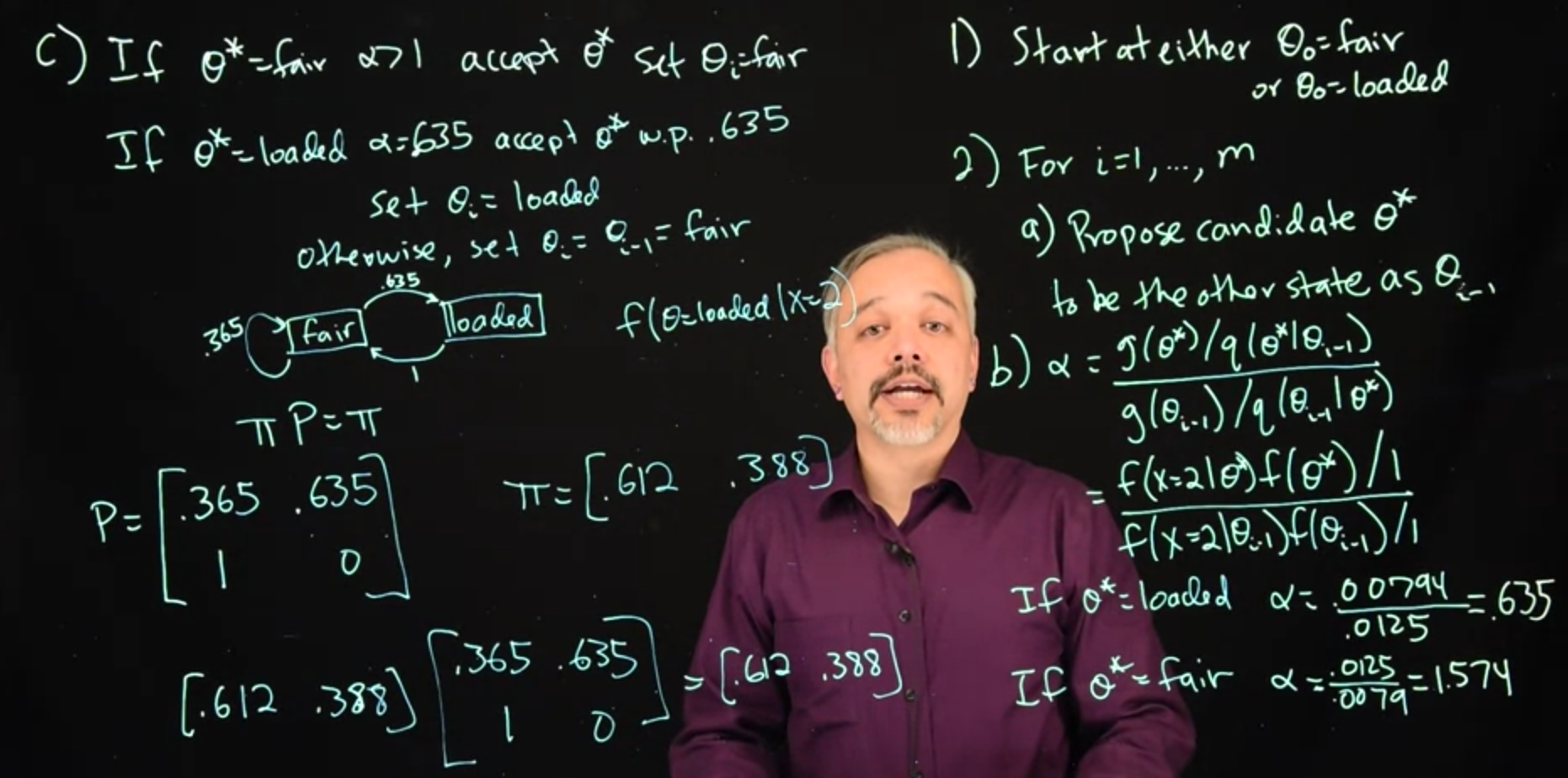
\begin{cases} \text{ accept } \theta^* \text { and set } \theta_i=\text{fair} & \text{If } \theta^*=\text{fair, } \alpha>1 \\ \begin{cases} \text{ accept } \theta^* \text{ and set } \theta_i=\text{loaded} & \text{ With probability } 0.635 \\ \text{ reject } \theta^* \text{ and set } \theta_i=\text{fair} & \text{ Otherwise } \end{cases} & \text{If } \theta^*=\text{loaded, } \alpha=.635 \end{cases}
If the \theta^*=\text{loaded} \implies \alpha=0.635. So we accept theta star with probability 0.635. And if we accept it. Set \theta_i=\text{loaded} Otherwise, set \theta_i = \theta_{i- 1}, if we do not accept, it stays in that same old fair state.
We can draw this out as a Markov chain with two states, Fair and ‘loaded’. If it’s in the ‘loaded’ state, it will move with probability one to the fair state. If it’s in the fair state, it will move with a probability of 0.635 to the ‘loaded’ state. And with a probability of 0.365 it will stay in the fair state.
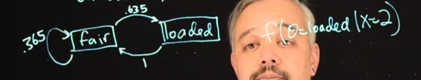
And so here’s a little diagram for this Markov chain with two states. In which case it will move back and forth with certain probabilities.
Thus, if we wanted to find our posterior probability , f(\theta=\text{loaded} \mid x=2). We can simulate from this Markov chain using these transition probabilities. And observe the fraction of time that it spends in the state theta equals ‘loaded’. And this gives us a good estimate of the posterior probability that it’s the ‘loaded’ coin. In this particular case, we can also show that this gives us the theoretical right answer.
If you’ve seen a little bit of the theory of Markov chains. We can say that a Markov chain with transition probability capital P, has stationary distribution \Pi.
\pi P = \pi \qquad \text{(def. stationary distribution)} \tag{33.7}
Here we have a transition probability matrix P, where we can think about ‘fair’ and ‘loaded’. Moving from the ‘fair’ state, remaining in the ‘fair’ state happens with a probability of 0.365 and it moves from ‘fair’ to ‘loaded’, with a probability of 0.635. If it’s in the ‘loaded’ state, we’ll move to the ‘fair’ state with probability one, and it will stay in the ‘loaded’ state with probability 0.
P= \begin{bmatrix} 0.365 & 0.635 \\ 1 & 0 \end{bmatrix}
In this case, we want our stationary distribution to be the posterior probabilities.
\Pi= \begin{bmatrix} 0.612 & 0.388 \\ \end{bmatrix}
Which you can recall are 0.612 of being ‘fair’ and 0.388 of being ‘loaded’. And so indeed, if you do just the minimal amount of matrix algebra, you can see that 0.612, 0.388 Multiplied by this matrix, 0.365, 0.635, 1, 0, does indeed give you 0.612 and 0.388, at least to within rounding error.
\begin{aligned} \Pi P &= \begin{bmatrix} 0.612 & 0.388 \end{bmatrix} \begin{bmatrix} 0.365 & 0.635 \\ 1 & 0 \end{bmatrix} \\ &= \begin{bmatrix} 0.612 & 0.388 \end{bmatrix} \\&= \Pi \end{aligned} \tag{33.8}
Thus in this case we can see, that we do get the correct stationary distribution for the Markov chain using the Metropolis–Hastings algorithm. And that when we simulate it, we do get correct estimates then of the posterior probabilities.
This is a nice simple example where we can work out the posterior probabilities in closed form. We don’t need to run Markov chain Monte Carlo. But this method is very powerful because all we need is to be able to evaluate the likelihood and the prior, we don’t need to evaluate the full posterior and get that normalizing constant. And so this applies to a much broader range of more complicated problems. Where we can use Markov chain Monte Carlo to simulate, to be able to get these probabilities. We’ll make good use of this in the rest of this course.
33.6 Random walk with Normal likelihood, t prior
Recall the model from the last segment of Lesson 2 where the data are the percent change in total personnel from last year to this year for n=10 companies. We used a normal likelihood with known variance and t distribution for the prior on the unknown mean. Suppose the values are y=(1.2,1.4,−0.5,0.3,0.9,2.3,1.0,0.1,1.3,1.9). Because this model is not conjugate, the posterior distribution is not in a standard form that we can easily sample. To obtain posterior samples, we will set up a Markov chain whose stationary distribution is this posterior distribution.
Recall that the posterior distribution is
\mathbb{P}r(\mu \mid y_1, \ldots, y_n) \propto \frac{\exp[ n ( \bar{y} \mu - \mu^2/2)]}{1 + \mu^2}
The posterior distribution on the left is our target distribution and the expression on the right is our g(\mu).
The first thing we can do in R is write a function to evaluate g(\mu). Because posterior distributions include likelihoods (the product of many numbers that are potentially small), g(\mu) might evaluate to such a small number that to the computer, it is effectively zero. This will cause a problem when we evaluate the acceptance ratio \alpha. To avoid this problem, we can work on the log scale, which will be more numerically stable. Thus, we will write a function to evaluate
\log(g(\mu)) = n ( \bar{y} \mu - \mu^2/2) - \log(1 + \mu^2)
This function will require three arguments, \mu, \bar{y}, and n.
Next, let’s write a function to execute the Random-Walk Metropolis-Hastings sampler with Normal proposals.
mh = function(n, ybar, n_iter, mu_init, cand_sd) {
  ## Random-Walk Metropolis-Hastings algorithm

  ## Step 1, initialize
  mu_out = numeric(n_iter)
  accpt = 0
  mu_now = mu_init
  lg_now = lg(mu=mu_now, n=n, ybar=ybar)

  ## Step 2, iterate
  for (i in 1:n_iter) {
    ## step 2a
    mu_cand = rnorm(n=1, mean=mu_now, sd=cand_sd) # draw a candidate

    ## Step 2b
    lg_cand = lg(mu=mu_cand, n=n, ybar=ybar) # evaluate log of g with the candidate
    lalpha = lg_cand - lg_now # log of acceptance ratio
    alpha = exp(lalpha)

    ## step 2c
    u = runif(1) # draw a uniform variable which will be less than alpha with probability min(1, alpha)
    if (u < alpha) { # then accept the candidate
      mu_now = mu_cand
      accpt = accpt + 1 # to keep track of acceptance
      lg_now = lg_cand
    }

    ## collect results
    mu_out[i] = mu_now # save this iteration's value of mu
  }

  ## return a list of output
  list(mu=mu_out, accpt=accpt/n_iter)
}
Now, let’s set up the problem.
y = c(1.2, 1.4, -0.5, 0.3, 0.9, 2.3, 1.0, 0.1, 1.3, 1.9)
ybar = mean(y)
n = length(y)
hist(y, freq=FALSE, xlim=c(-1.0, 3.0)) # histogram of the data
curve(dt(x=x, df=1), lty=2, add=TRUE) # prior for mu
points(y, rep(0,n), pch=1) # individual data points
points(ybar, 0, pch=19) # sample mean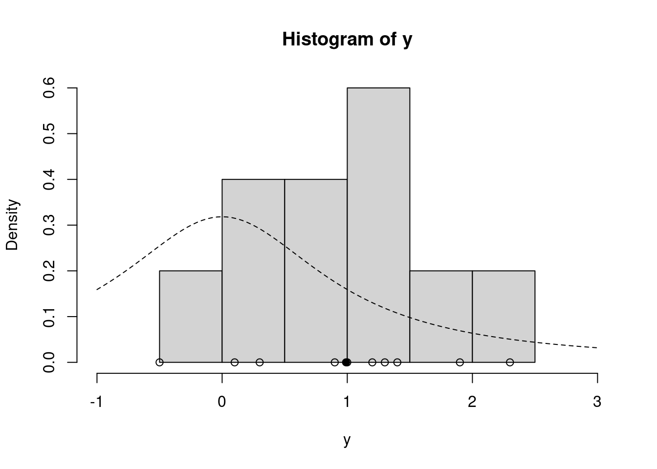
Finally, we’re ready to run the sampler! Let’s use m=1000 iterations and proposal standard deviation (which controls the proposal step size) 3.0, and initial value at the prior median 0.
set.seed(43) # set the random seed for reproducibility
post = mh(n=n, ybar=ybar, n_iter=1e3, mu_init=0.0, cand_sd=3.0)
str(post)
List of 2
$ mu : num [1:1000] -0.113 1.507 1.507 1.507 1.507 ...
$ accpt: num 0.122library("coda")
traceplot(as.mcmc(post$mu))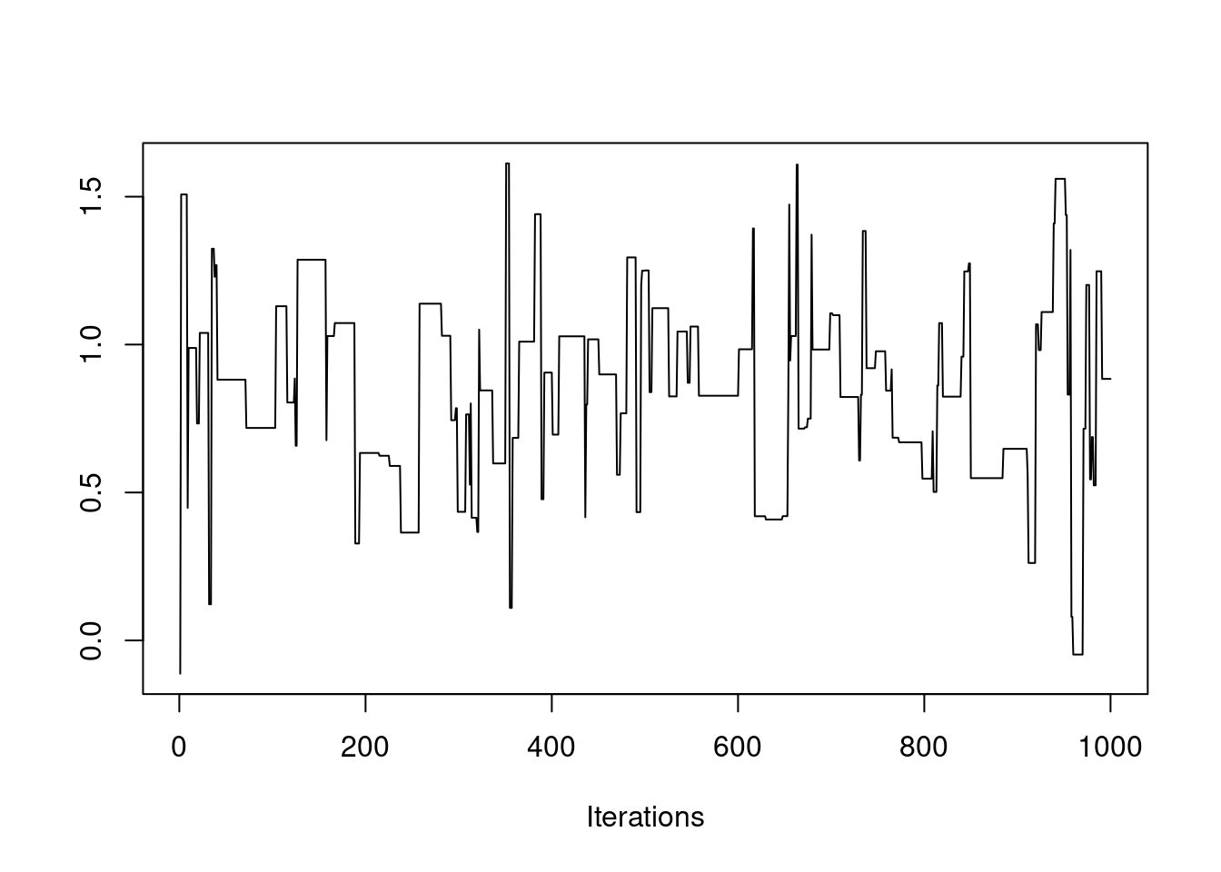
This last plot is called a trace plot. It shows the history of the chain and provides basic feedback about whether the chain has reached its stationary distribution.
It appears our proposal step size was too large (acceptance rate below 23%). Let’s try another.
post = mh(n=n, ybar=ybar, n_iter=1e3, mu_init=0.0, cand_sd=0.05)
post$accpt
[1] 0.946traceplot(as.mcmc(post$mu))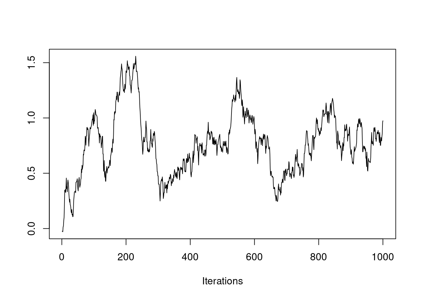
Oops, the acceptance rate is too high (above 50%). Let’s try something in between.
post = mh(n=n, ybar=ybar, n_iter=1e3, mu_init=0.0, cand_sd=0.9)
post$accpt
[1] 0.38traceplot(as.mcmc(post$mu))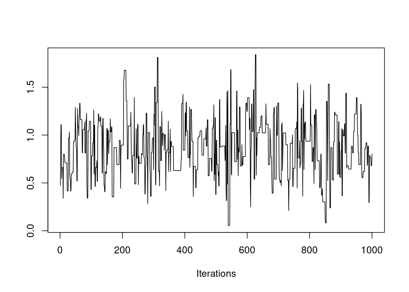
Which looks good. Just for fun, let’s see what happens if we initialize the chain at some far-off value.
post = mh(n=n, ybar=ybar, n_iter=1e3, mu_init=30.0, cand_sd=0.9)
post$accpt
[1] 0.387traceplot(as.mcmc(post$mu))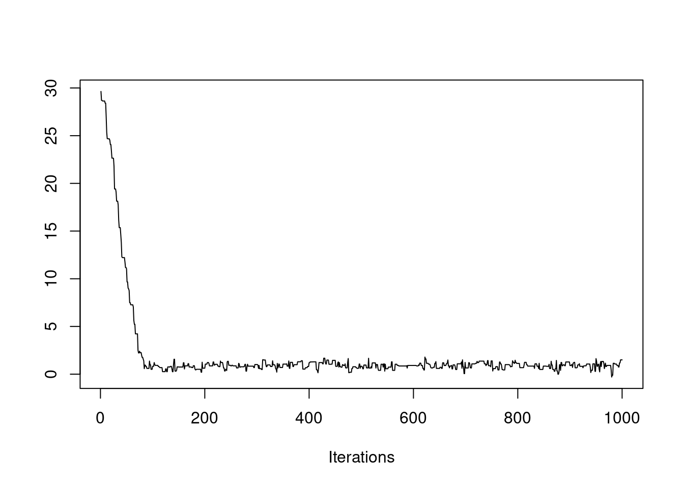
It took awhile to find the stationary distribution, but it looks like we succeeded! If we discard the first 100 or so values, it appears like the rest of the samples come from the stationary distribution, our posterior distribution! Let’s plot the posterior density against the prior to see how the data updated our belief about \mu.
post$mu_keep = post$mu[-c(1:100)] # discard the first 200 samples
plot(density(post$mu_keep, adjust=2.0), main="", xlim=c(-1.0, 3.0), xlab=expression(mu)) # plot density estimate of the posterior
curve(dt(x=x, df=1), lty=2, add=TRUE) # prior for mu
points(ybar, 0, pch=19) # sample mean

curve(0.017*exp(lg(mu=x, n=n, ybar=ybar)), from=-1.0, to=3.0, add=TRUE, col="blue") # approximation to the true posterior in blue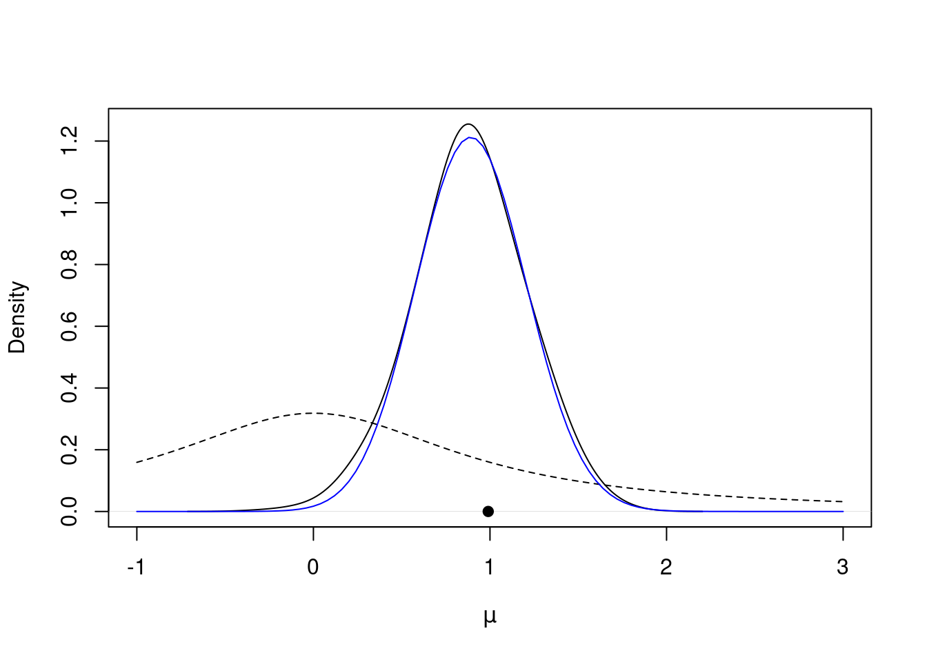
These results are encouraging, but they are preliminary. We still need to investigate more formally whether our Markov chain has converged to the stationary distribution. We will explore this in a future lesson.
Obtaining posterior samples using the Metropolis-Hastings algorithm can be time-consuming and require some fine-tuning, as we’ve just seen. The good news is that we can rely on software to do most of the work for us. In the next couple of videos, we’ll introduce a program that will make posterior sampling easy.
34 Introduction to JAGS
34.1 Setup
34.1.1 Introduction to JAGS
There are several software packages available that will handle the details of MCMC for us. See the supplementary material for a brief overview of options.
The package we will use in this course is JAGS (Just Another Gibbs Sampler) by Martyn Plummer. The program is free, and runs on Mac OS, Windows, and Linux. Better yet, the program can be run using R with the rjags and R2jags packages.
In JAGS, we can specify models and run MCMC samplers in just a few lines of code; JAGS does the rest for us, so we can focus more on the statistical modeling aspect and less on the implementation. It makes powerful Bayesian machinery available to us as we can fit a wide variety of statistical models with relative ease.
34.1.2 Installation and setup
The starting place for JAGS users is mcmc-jags.sourceforge.net. At this site, you can find news about the features of the latest release of JAGS, links to program documentation, as well as instructions for installation.
The documentation is particularly important. It is available under the files page link in the Manuals folder.
Also under the files page, you will find the JAGS folder where you can download and install the latest version of JAGS. Select the version and operating system, and follow the instructions for download and installation.
Once JAGS is installed, we can immediately run it from R using the rjags package. The next segment will show how this is done.
34.2 Modeling in JAGS
There are four steps to implementing a model in JAGS through R:
- Specify the model.
- Set up the model.
- Run the MCMC sampler.
- Post-processing.
We will demonstrate these steps with our running example with the data are the percent change in total personnel from last year to this year for n=10 companies. We used a normal likelihood with known variance and t distribution for the prior on the unknown mean.
34.2.1 1. Specify the model
In this step, we give JAGS the hierarchical structure of the model, assigning distributions to the data (the likelihood) and parameters (priors). The syntax for this step is very similar to R, but there are some key differences.
library("rjags")Linked to JAGS 4.3.2Loaded modules: basemod,bugsmod_string = " model {
for (i in 1:n) {
y[i] ~ dnorm(mu, 1.0/sig2)
}
mu ~ dt(0.0, 1.0/1.0, 1.0) # location, inverse scale, degrees of freedom
sig2 = 1.0
} "One of the primary differences between the syntax of JAGS and R is how the distributions are parameterized. Note that the normal distribution uses the mean and precision (instead of variance). When specifying distributions in JAGS, it is always a good idea to check the JAGS user manual here in the chapter on Distributions.
34.2.2 2. Set up the model
set.seed(50)
y = c(1.2, 1.4, -0.5, 0.3, 0.9, 2.3, 1.0, 0.1, 1.3, 1.9)
n = length(y)

data_jags = list(y=y, n=n)
params = c("mu")

inits = function() {
  inits = list("mu"=0.0)
} # optional (and fixed)

mod = jags.model(textConnection(mod_string), data=data_jags, inits=inits)
Compiling model graph
Resolving undeclared variables
Allocating nodes
Graph information:
Observed stochastic nodes: 10
Unobserved stochastic nodes: 1
Total graph size: 15
Initializing modelThere are multiple ways to specify initial values here. They can be explicitly set, as we did here, or they can be random, i.e., list("mu"=rnorm(1)). Also, we can omit the initial values, and JAGS will provide them.
34.2.3 3. Run the MCMC sampler
update(mod, 500) # burn-in

mod_sim = coda.samples(model=mod, variable.names=params, n.iter=1000)
We will discuss more options to the coda.samples function in coming examples.
34.2.4 4. Post-processing
summary(mod_sim)
Iterations = 1501:2500
Thinning interval = 1
Number of chains = 1
Sample size per chain = 1000

1. Empirical mean and standard deviation for each variable,
   plus standard error of the mean:

          Mean             SD       Naive SE Time-series SE
      0.888698       0.311080       0.009837       0.012007

2. Quantiles for each variable:

  2.5%    25%    50%    75%  97.5%
0.2964 0.6767 0.8775 1.0968 1.5256 library("coda")
plot(mod_sim)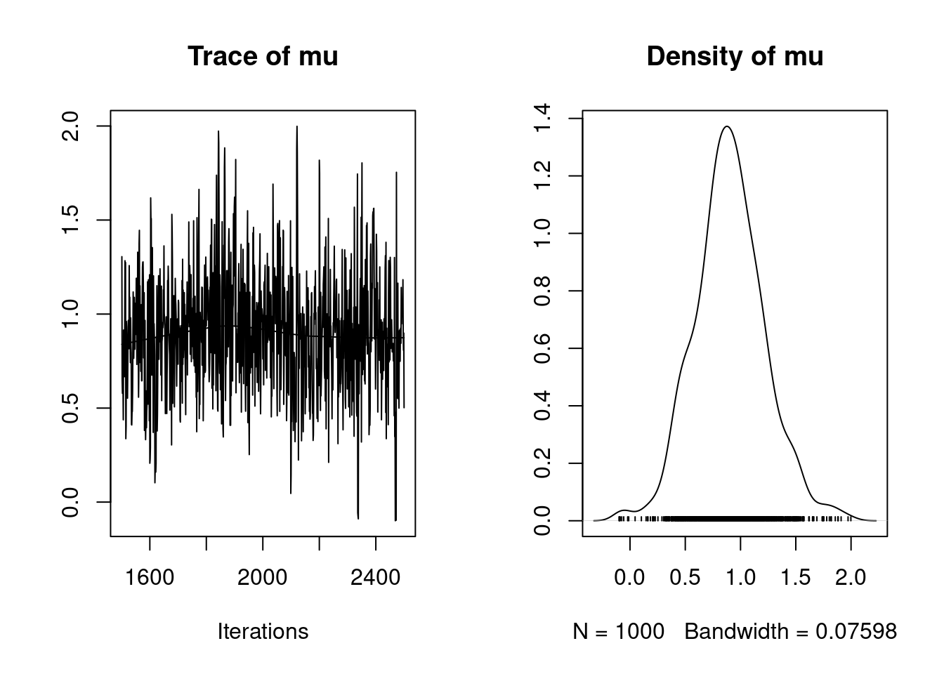
We will discuss post processing further, including convergence diagnostics, in a coming lesson.