---
date: 2024-11-05
title: "Bayesian Inference in the AR($p$) - M2L5"
subtitle: "Time Series Analysis"
description: "The AR($p$) process, its state-space representation, the characteristic polynomial, and the forecast function"
categories: [Coursera, notes, Bayesian Statistics, Autoregressive Models, Time Series]
keywords: [time series, AR(p), Bayesian inference, State Space Model, ARIMA, R code, Characteristic lag polynomial, autocorrelation function, ACF, partial autocorrelation function, PACF, smoothing, ARMA process, moving average]
---
## Bayesian inference in the AR($p$): Reference prior, conditional likelihood :movie_camera:
{#fig-ar-p-process .column-margin group="slides" width="53mm"}
### Model Setup
we start with an **AR($p$)** model as we define in the previous lesson:
$$
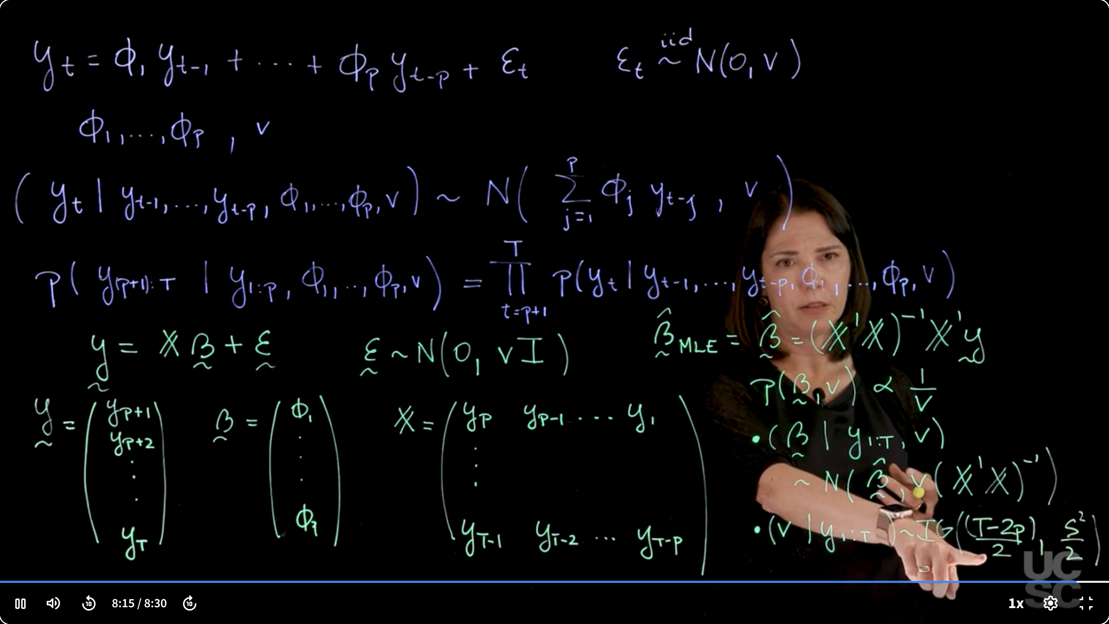
y_t = \phi_1 y_{t-1} + \ldots + \phi_p y_{t-p} + \varepsilon_t \qquad \varepsilon_t \stackrel{iid}{\sim} \mathcal{N}(0, \nu)
$$ {#eq-arp-inf-model}
- We wish to infer:
- $\phi_i$ the *AR($p$)* coefficients and
- $\nu$ the innovation variance.
### Conditional likelihood
We make use of the autoregressive structure and rewrite $y_t$ conditionally on the previous $p$ values of the process and the parameters:
$$
(y_t \mid y_{t-1}, \ldots, y_{t-p}, \phi_1, \ldots, \phi_p) \sim \mathcal{N}\left (\sum_{j=1}^{p} \phi_j y_{t-j}, v\right )
$$ {#eq-arp-inf-cond}
[We condition on the first $p$ values of the process.]{.mark}
The conditional distribution of $y_t$ given the previous $p$ values and parameters is normal with mean given by the weighted sum $\sum \phi_j y_{t-j}$ and variance $v$.
the density for the first $p$ observations is given by:
$$
\mathbb{P}r(y_{(p+1):T}\mid y_{1:p}, \phi_1, \ldots, \phi_p, v) = \prod_{t=p+1}^{T} \mathbb{P}r(y_t \mid y_{t-1}, \ldots, y_{t-p}, \phi_1, \ldots, \phi_p, v)
$$ {#eq-arp-inf-full-cond-likelihood}
This product of conditionals yields the full conditional likelihood.
Each term is Gaussian and independent, given the past values and parameters.
### Regression Formulation
This is recast as a linear regression: response vector $\mathbf{y}$ starting from $y_{p+1}$ to $y_T$, design matrix $\mathbb{X}$ built from lagged values, and $\boldsymbol\beta$ as the AR coefficients $\phi_j$.
$$
\mathbf{y}= \mathbb{X}\boldsymbol \beta + \boldsymbol \varepsilon \qquad \varepsilon \sim \mathcal{N}(0, vI)
$$ {#eq-arp-inf-regression}
$$
\mathbf{y} = \begin{pmatrix} y_{p+1} \\ y_{p+2} \\ \vdots \\ y_T \end{pmatrix}, \quad
\boldsymbol \beta = \begin{pmatrix} \phi_1 \\ \phi_2 \\ \vdots \\ \phi_p \end{pmatrix}, \quad
\mathbb{X} = \begin{pmatrix} y_{p} & y_{p-1} & \cdots & y_{1} \\ y_{p+1} & y_{p} & \cdots & y_{2} \\ \vdots & \vdots & \ddots & \vdots \\ y_{T-1} & y_{T-2} & \cdots & y_{T-p} \end{pmatrix}
$$
In the design matrix $\mathbb{X}$ each row corresponds to lagged observations used to predict the next value. This setup enables applying linear regression machinery.
Assuming full-rank $\mathbb{X}$, we may now infer the parameters by using the left generalized Moore-Penrose inverse of $\mathbb{X}$ as the maximum likelihood estimator (MLE) of the AR coefficients $\boldsymbol \beta$.
$$
\boldsymbol \beta_{MLE} = (\mathbb{X}^\top \mathbb{X})^{-1} \mathbb{X}^\top \mathbf{y}
$$ {#eq-arp-inf-regression-mle}
where:
- $\mathbb{X}$ is the design matrix,
- $\boldsymbol \beta$ is the vector of AR coefficients, and
- $\mathbf{y}$ is the response vector.
It matches the usual OLS solution in linear regression.
### Reference prior and posterior distribution
The reference prior reflects non-informative beliefs. This yields a conjugate posterior due to the Gaussian likelihood.
$$
p(\beta,v) \propto 1/v
$$ {#eq-arp-inf-prior}
$$
(\boldsymbol \beta \mid \mathbf{y}_{:T}, v) \sim \mathcal{N}(\boldsymbol \beta_{MLE}, v (\mathbb{X}^\top \mathbb{X})^{-1})
$$ {#eq-arp-inf-posterior-beta}
The posterior is Gaussian with mean $\boldsymbol \beta_{MLE}$ and scaled covariance $v(\mathbb{X}^\top \mathbb{X})^{-1}$, analogous to the OLS variance.
$$
(v \mid \mathbf{y}_{:T}) \sim \text{Inverse-Gamma}\left(\frac{T - 2p}{2}, \frac{S^2}{2}\right)
$$ {#eq-arp-inf-posterior-v}
where:
- $S^2 = \sum_{t=p+1}^{T} (y_t - \mathbb{X} \boldsymbol \beta_{MLE})^2$ is the unbiased estimator of the variance $v$.
- $T$ is the total number of observations.
Posterior for $v$ is inverse gamma. The shape parameter is $(T - 2p)/2$ because the number of residual degrees of freedom is $T - 2p$ (residual = $T-p$ obs minus $p$ params). Scale is half the sum of squared residuals.
### Simulation-based Inference
Posterior sampling:
- Draw $v$ from the inverse gamma posterior.
- Plug $v$ into the posterior of $\boldsymbol\beta$ and sample from the Gaussian.
This gives full Bayesian posterior samples of $(\boldsymbol\beta, v)$.
### Summary
- In this lesson, we discussed the Bayesian inference for the *AR($p$)* process using the conditional likelihood and reference prior.
- We have established a connection between the *AR($p$)* process and a regression model, allowing us to use standard regression techniques to estimate the parameters.
- The posterior distribution can be derived, and we can perform simulation-based inference to obtain samples from the posterior distribution of the AR coefficients and variance.
::: {.callout-note collapse="true"}
## Video Transcript {.unnumbered}
{{< include transcripts/_C4-L05-T01.qmd >}}
:::
## R code: Maximum likelihood estimation, AR($p$), conditional likelihood :spiral_notepad:
\index{Maximum Likelihood Estimation}
```{r}
#| label: ar-likelihood
  set.seed(2021)
# Simulate 300 observations from an AR(2) with one pair of complex-valued reciprocal roots
r=0.95
lambda=12
phi=numeric(2)
phi[1]=2*r*cos(2*pi/lambda)
phi[2]=-r^2
sd=1 # innovation standard deviation
T=300 # number of time points
# generate stationary AR(2) process
yt=arima.sim(n = T, model = list(ar = phi), sd = sd)

## Compute the MLE for phi and the unbiased estimator for v using the conditional likelihood
p=2
y=rev(yt[(p+1):T]) # response
X=t(matrix(yt[rev(rep((1:p),T-p)+rep((0:(T-p-1)),rep(p,T-p)))],p,T-p));
XtX=t(X)%*%X
XtX_inv=solve(XtX)
phi_MLE=XtX_inv%*%t(X)%*%y # MLE for phi
s2=sum((y - X%*%phi_MLE)^2)/(length(y) - p) #unbiased estimate for v

cat("\n MLE of conditional likelihood for phi: ", phi_MLE, "\n",
    "Estimate for v: ", s2, "\n")
```
## Model order selection :movie_camera: {#sec-arp-order-selection}
{#fig-ar-p-model-order-selection .column-margin group="slides" width="53mm"}
### Goal
Determine the best model order $p$ for an AR($p$) process by comparing candidate models.
### Step 1: Define a candidate set of model orders
$$
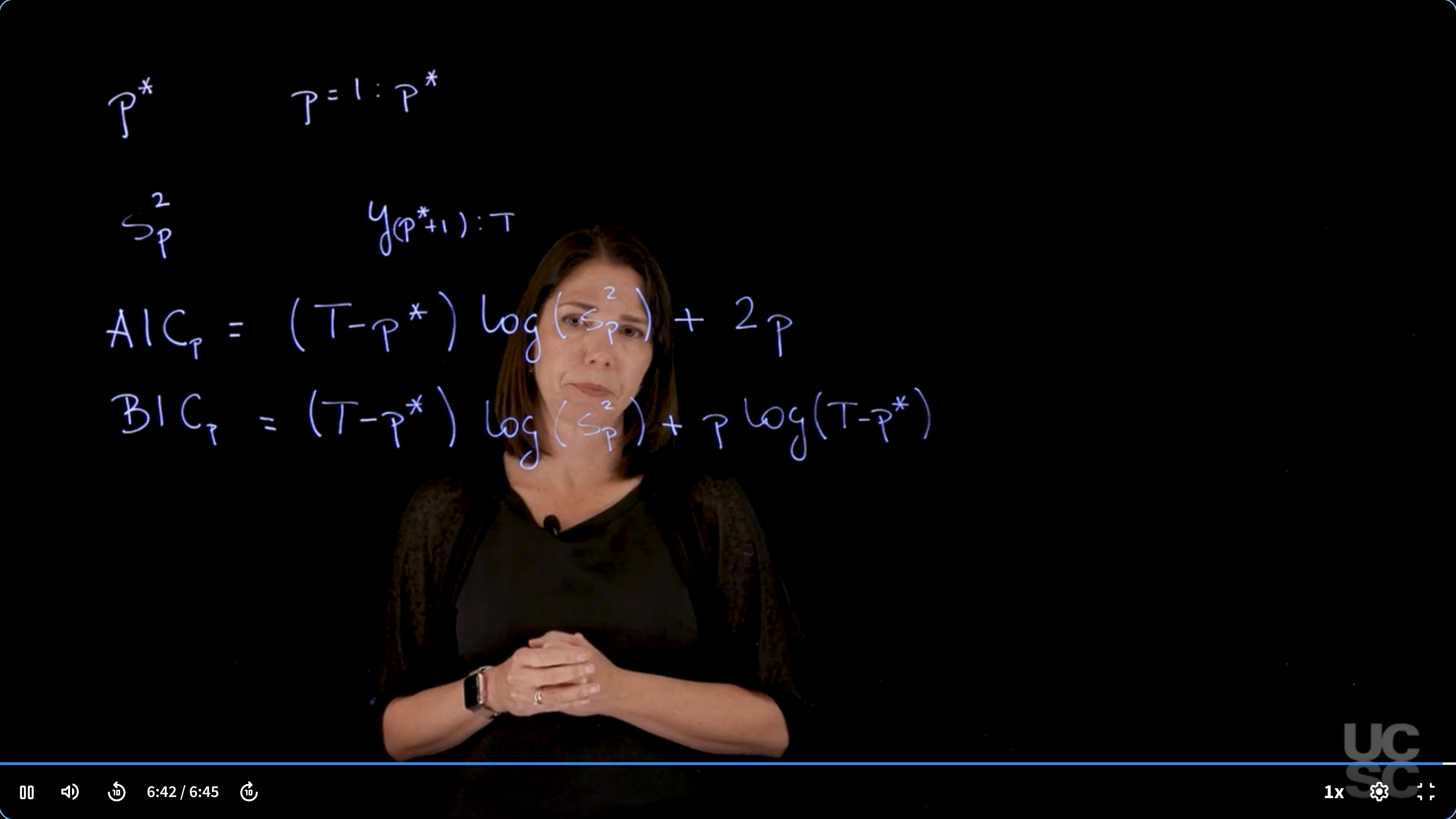
p^* \qquad p=1:p^*
$$
You choose a maximum order $p^*$ (e.g., 20), then evaluate AR models of each order $p \in {1, \dots, p^*}$.
### Step 2: Estimate residual variance for each model
$$
S^2_p \qquad y_{(p^*+1):T}
$$
For each model of order $p$, compute $S_p^2$ as the residual sum of squares (RSS) using a fixed evaluation window: $t = p^*+1$ to $T$, to ensure all models are evaluated on the same data subset.
### Step 3: Compute model selection criteria
\index{model selection}
\index{model selection!AIC}
\index{model selection!BIC}
\index{Aikaike Information Criterion}
\index{Bayesian Information Criterion}
AIC balances fit (log-likelihood) with complexity (number of parameters).
The first term measures model fit using $\log(S_p^2)$, and the second term penalizes complexity with $2p$.
$$
AIC_p = (T-p^*) \log(S_p^2) + 2p
$$
BIC uses the same fit term but a heavier penalty: $p \log(T - p^*)$, which increases with sample size. This often leads BIC to favor smaller models than AIC.
$$
BIC_p = (T-p^*) \log(S_p^2) + p \log(T-p^*)
$$
::: {.callout-note collapse="true"}
## Video Transcript {.unnumbered}
{{< include transcripts/_C4-L05-T02.qmd >}}
:::
## Example: Bayesian inference in the AR($p$), conditional likelihood :movie_camera:
This video walks through the code in the next section which demonstrates Bayesian inference for an AR(2) process with complex-valued roots.
::: {.callout-note collapse="true"}
## Video Transcript {.unnumbered}
{{< include transcripts/_C4-L05-T03.qmd >}}
:::
## code: Bayesian inference, AR($p$), conditional likelihood :spiral_notepad: $\mathcal{R}${#sec-arp-bayesian-inference}
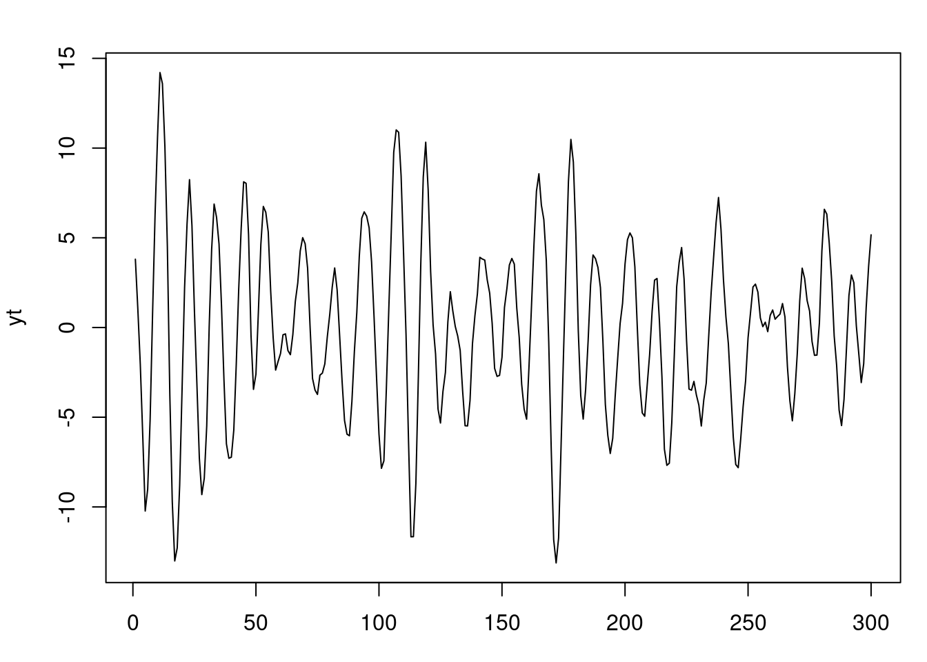
### Simulate 300 observations from an AR(2) with one pair of complex-valued roots
```{r}
#| label: fig-ar-bayesian-inference
#| fig-cap: Simulated AR(2) process with complex-valued roots
set.seed(2021)
r=0.95
lambda=12
phi=numeric(2)
phi[1]=2*r*cos(2*pi/lambda)
phi[2]=-r^2
sd=1 # innovation standard deviation
T=300 # number of time points
# generate stationary AR(2) process
yt=arima.sim(n = T, model = list(ar = phi), sd = sd)

par(mfrow=c(1,1), mar = c(3, 4, 2, 1) )
plot(yt)
```
### Compute the MLE of phi and the unbiased estimator of v using the conditional likelihood
```{r}
#| label: ar-bayesian-inference-mle
p=2
y=rev(yt[(p+1):T]) # response
X=t(matrix(yt[rev(rep((1:p),T-p)+rep((0:(T-p-1)),rep(p,T-p)))],p,T-p));
XtX=t(X)%*%X
XtX_inv=solve(XtX)
phi_MLE=XtX_inv%*%t(X)%*%y # MLE for phi
phi_MLE
s2=sum((y - X%*%phi_MLE)^2)/(length(y) - p) #unbiased estimate for v
s2
```
### Posterior inference, conditional likelihood + reference prior via direct sampling
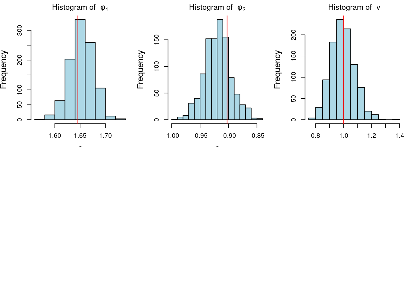
```{r}
#| label: fig-ar-bayesian-inference-posterior
#| fig-cap: Posterior distributions of AR(2) parameters
n_sample=1000 # posterior sample size
library(MASS)

## step 1: sample v from inverse gamma distribution
v_sample=1/rgamma(n_sample, (T-2*p)/2, sum((y-X%*%phi_MLE)^2)/2)

## step 2: sample phi conditional on v from normal distribution
phi_sample=matrix(0, nrow = n_sample, ncol = p)
for(i in 1:n_sample){
  phi_sample[i, ]=mvrnorm(1,phi_MLE,Sigma=v_sample[i]*XtX_inv)
}

par(mfrow = c(2, 3), mar = c(3, 4, 2, 1),  cex.lab = 1.3)
## plot histogram of posterior samples of phi and v

for(i in 1:2){
  hist(phi_sample[, i], xlab = bquote(phi),
       main = bquote("Histogram of "~phi[.(i)]),col='lightblue')
  abline(v = phi[i], col = 'red')
}

hist(v_sample, xlab = bquote(nu), main = bquote("Histogram of "~v),col='lightblue')
abline(v = sd, col = 'red')
```
### Graph posterior for modulus and period
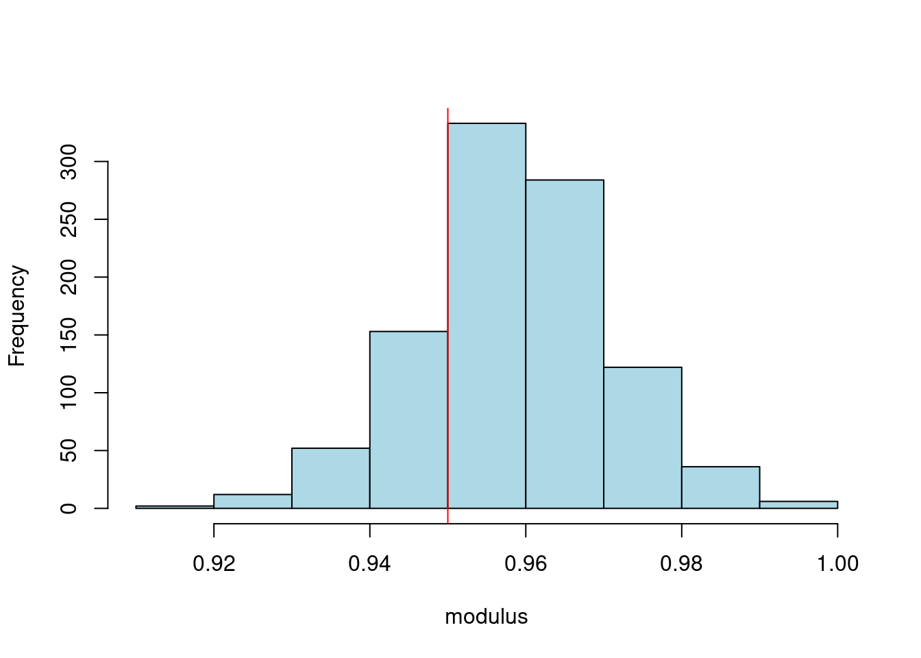
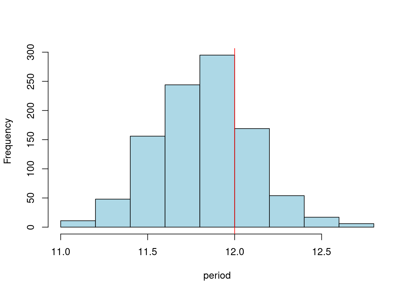
```{r}
#| label: fig-ar-bayesian-inference-roots
#| fig-cap: Posterior distributions of AR(2) roots
#| fig-subcap:
#| - modulus
#| - period
#| layout-ncol: 2
r_sample=sqrt(-phi_sample[,2])
lambda_sample=2*pi/acos(phi_sample[,1]/(2*r_sample))

hist(r_sample,xlab="modulus",main="",col='lightblue')
abline(v=0.95,col='red')

hist(lambda_sample,xlab="period",main="",col='lightblue')
abline(v=12,col='red')
```
## code: Model order selection :spiral_notepad: $\mathcal{R}$ {#sec-ar-2-model-order-selection}
### Simulate data from an AR(2)
```{r}
#| label: fig-ar-2-model-order-selection-simulation
#| fig-cap: Simulated AR(2) process with complex-valued roots
set.seed(2021)
r=0.95
lambda=12
phi=numeric(2)
phi[1]=2*r*cos(2*pi/lambda)
phi[2]=-r^2
sd=1 # innovation standard deviation
T=300 # number of time points
# generate stationary AR(2) process
yt=arima.sim(n = T, model = list(ar = phi), sd = sd)
par(mfrow=c(1,1), mar = c(3, 4, 2, 1) )
plot(yt)
```
### compute MLE for different AR($p$)s
```{r}
#| label: ar-2-model-order-selection-MLE
pmax=10 # the maximum of model order
Xall=t(matrix(yt[rev(rep((1:pmax),T-pmax)+rep((0:(T-pmax-1)),
              rep(pmax,T-pmax)))], pmax, T-pmax));
y=rev(yt[(pmax+1):T])
n_cond=length(y) # (number of total time points - the maximum of model order)

## compute MLE
my_MLE <- function(y, Xall, p){
  n=length(y)
  x=Xall[,1:p]
  a=solve(t(x) %*%x)
  a=(a + t(a))/2 # for numerical stability
  b=a%*%t(x)%*%y # mle for ar coefficients
  r=y - x%*%b # residuals
  nu=n - p # degrees freedom
  R=sum(r*r) # SSE
  s=R/nu #MSE
  return(list(b = b, s = s, R = R, nu = nu))
}
```
### Compute AIC and BIC for different AR($p$)s based on simulated data
```{r}
## function for AIC and BIC computation
AIC_BIC <- function(y, Xall, p){
  ## number of time points
  n <- length(y)

  ## compute MLE
  tmp=my_MLE(y, Xall, p)

  ## retrieve results
  R=tmp$R

  ## compute likelihood
  likl= n*log(R)

  ## compute AIC and BIC
  aic =likl + 2*(p)
  bic =likl + log(n)*(p)
  return(list(aic = aic, bic = bic))
}
# Compute AIC, BIC
aic =numeric(pmax)
bic =numeric(pmax)

for(p in 1:pmax){
  tmp =AIC_BIC(y,Xall, p)
  aic[p] =tmp$aic
  bic[p] =tmp$bic
  print(c(p, aic[p], bic[p])) # print AIC and BIC by model order
}
## compute difference between the value and its minimum
aic =aic-min(aic)
aic
bic =bic-min(bic)
bic
```
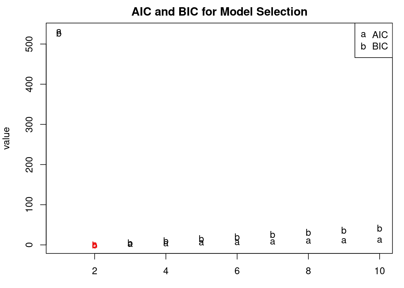
### Plot AIC, BIC, and the marginal likelihood
```{r}
#| label: fig-ar-2-model-order-selection-plot
#| fig-cap: AIC, BIC for different AR($p$) model orders
par(mfrow = c(1, 1), mar = c(3, 4, 2, 1) )
matplot(1:pmax,matrix(c(aic,bic),pmax,2),ylab='value',
        xlab='AR order p',pch="ab", col = 'black', main = "AIC and BIC for Model Selection")
# highlight the model order selected by AIC
text(which.min(aic), aic[which.min(aic)], "a", col = 'red')
# highlight the model order selected by BIC
text(which.min(bic), bic[which.min(bic)], "b", col = 'red')

legend("topright", legend = c("AIC", "BIC"), col = c("black", "black"), pch = c("a", "b"))

p <- which.min(bic) # We set up the moder order
print(paste0("The chosen model order by BIC: ", p))
```
## Spectral representation of the AR($p$) :movie_camera:
{#fig-ar-p-spectral-representation .column-margin group="slides" width="53mm"}
The spectral representation of the *AR($p$)* process is a powerful tool for understanding the frequency domain properties of the process. It allows us to analyze how the process behaves at different frequencies and provides insights into its periodicity and persistence.
Supose we have an *AR($p$)* process with parameters:
$$
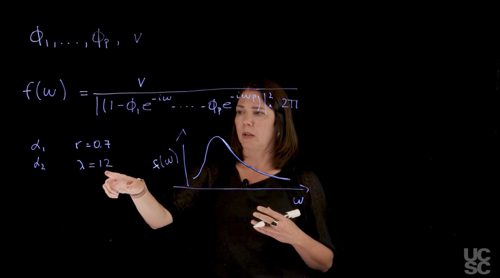
\phi_1, \ldots, \phi_2, v
$$
Properties related to the autocorrelation function of the process, and the forecast function as well as we have seen, are related to the reciprocal roots of the characteristic polynomial.
Using this information, we can also obtain a spectral representation of the process, meaning a representation in the frequency domain. We can think of this as a [density in the frequency domain where you’re going to have a power associated to different frequencies.]{.mark} In the case of an *AR($p$)* process, I can write down the spectral density of the process, as:
$$
f(\omega) = \frac{v}{ \mid 1 - \phi_1 e^{-i\omega} - \ldots - \phi_p e^{-i \omega p}) \mid^2 2\pi}
$$
with:
- $\omega \in [0,\pi]$ the frequency
For instance, if you have an AR(2), an autoregressive process of order 2, and you happen to have a pair of complex roots. Let’s assume that the reciprocal roots are $\alpha_1, \alpha_2$ with modulus $r$ and period $\lambda$, then the spectral density of the AR(2) process is given by:
$$
\alpha_1 \qquad r=0.7
$$
$$
\alpha_2 \qquad \lambda=12
$$
::: {.callout-note collapse="true"}
## Video Transcript {.unnumbered}
{{< include transcripts/_C4-L05-T04.qmd >}}
:::
## Spectral representation of the AR($p$): Example :movie_camera:
This video walks through the code in the next section.
### Summary: Posterior Spectral Density Estimation for AR(2)
* **Goal**: Estimate and visualize the **spectral density** of an AR(2) process and its **posterior distribution** based on observed data.
* **Simulation**: 300 observations are drawn from an AR(2) process with **complex conjugate roots** of modulus 0.95 and **period 12**, leading to a quasi-periodic process.
* **Estimation**:
* AR coefficients estimated via **MLE**.
* Innovation variance $v$ estimated as $s^2$ (unbiased).
* Posterior samples:
* $v \sim \text{Inverse-Gamma}$
* $\boldsymbol\Phi \mid v \sim \text{Bivariate Normal}$
* **Spectral density estimation**:
* `spec.ar()`: Uses MLEs to estimate the spectral density.
* `arma.spec()` from `astsa`: Allows using arbitrary (MLE or posterior) estimates of AR coefficients and variance.
* Accepts **posterior samples**, producing a distribution of spectral density curves.
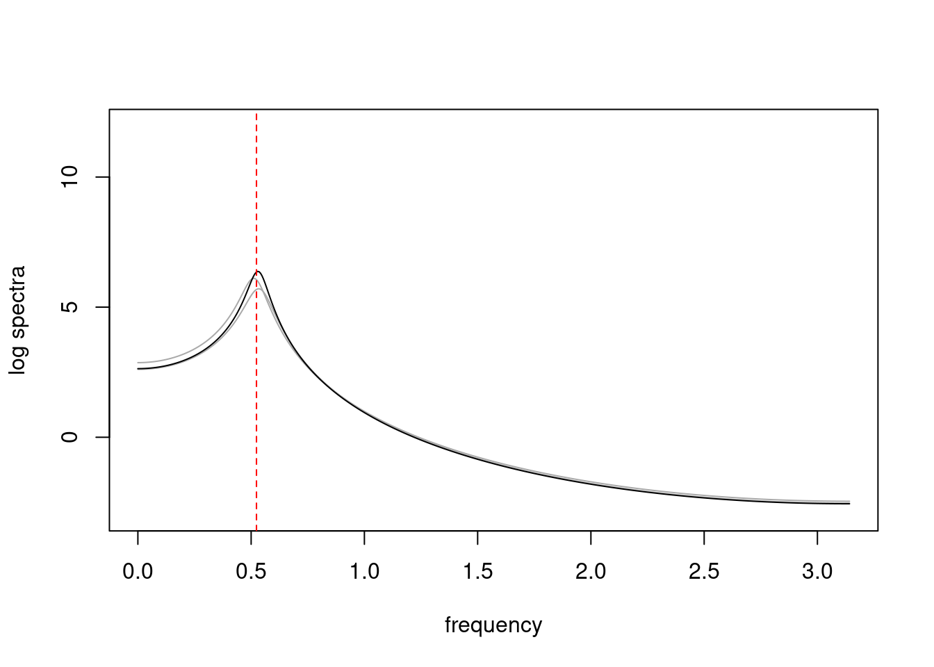
* **Results**:
* Plots show a **spectral peak at period 12**, as expected from the simulation.
* Posterior spectral densities are overlaid.
* **Solid line** = MLE-based spectrum; **dotted line** = true spectrum peak.
\index{AR($p$)!spectral density estimation}
\index{AR($p$)!frequency-domain}
This process illustrates Bayesian uncertainty in frequency-domain features of AR processes.
::: {.callout-note collapse="true"}
## Video Transcript {.unnumbered}
{{< include transcripts/_C4-L05-T05.qmd >}}
:::
## code: Spectral density of AR($p$) :spiral_notepad: $\mathcal{R}$
\index{AR($p$)!spectral density}
We will now obtain the spectral density of an autoregressive process, as well as visualize posterior distributions of the spectral densities of this AR process just based on data that we have
Simulate 300 observations from an *AR(2)* process with a pair of complex-valued roots
```{r}
#| label: ar-spectral-density
set.seed(2021)
r=0.95
lambda=12
phi=numeric(2)
phi[1]<- 2*r*cos(2*pi/lambda)
phi[2] <- -r^2
sd=1 # innovation standard deviation
T=300 # number of time points
# sample from the AR(2) process
yt=arima.sim(n = T, model = list(ar = phi), sd = sd)
```
Compute the MLE of $\phi$ and the unbiased estimator of $v$ using the conditional likelihood
```{r}
#| label: ar-spectral-density-mle
p=2
y=rev(yt[(p+1):T])
X=t(matrix(yt[rev(rep((1:p),T-p)+rep((0:(T-p-1)),rep(p,T-p)))],p,T-p));
XtX=t(X)%*%X
XtX_inv=solve(XtX)
phi_MLE=XtX_inv%*%t(X)%*%y # MLE for phi
s2=sum((y - X%*%phi_MLE)^2)/(length(y) - p) #unbiased estimate for v
```
Obtain 200 samples from the posterior distribution under the conditional likelihood and the reference prior and the direct sampling method
```{r}
#| label: ar-spectral-density-posterior
#| fig-cap: Posterior samples
n_sample=200 # posterior sample size
library(MASS)

## step 1: sample v from inverse gamma distribution
v_sample=1/rgamma(n_sample, (T-2*p)/2, sum((y-X%*%phi_MLE)^2)/2)

## step 2: sample phi conditional on v from normal distribution
phi_sample=matrix(0, nrow = n_sample, ncol = p)
for(i in 1:n_sample){
  phi_sample[i,]=mvrnorm(1,phi_MLE,Sigma=v_sample[i]*XtX_inv)
}
```
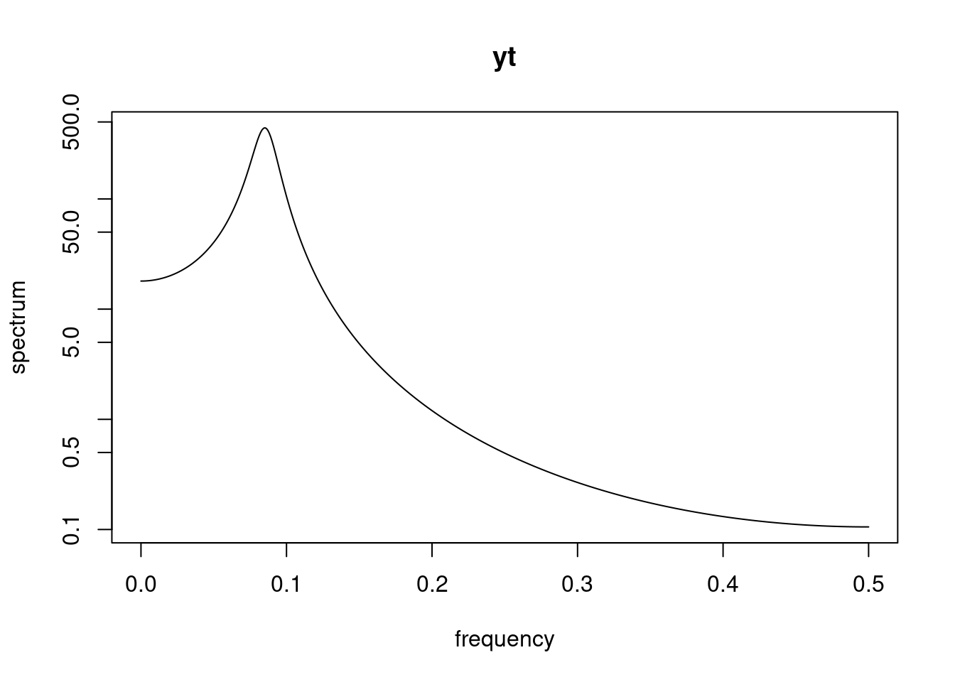
using `spec.ar` to draw spectral density based on the data assuming an AR(2)
```{r}
#| label: ar-spectral-density-spec-ar
spec.ar(yt, order = 2, main = "yt")
```
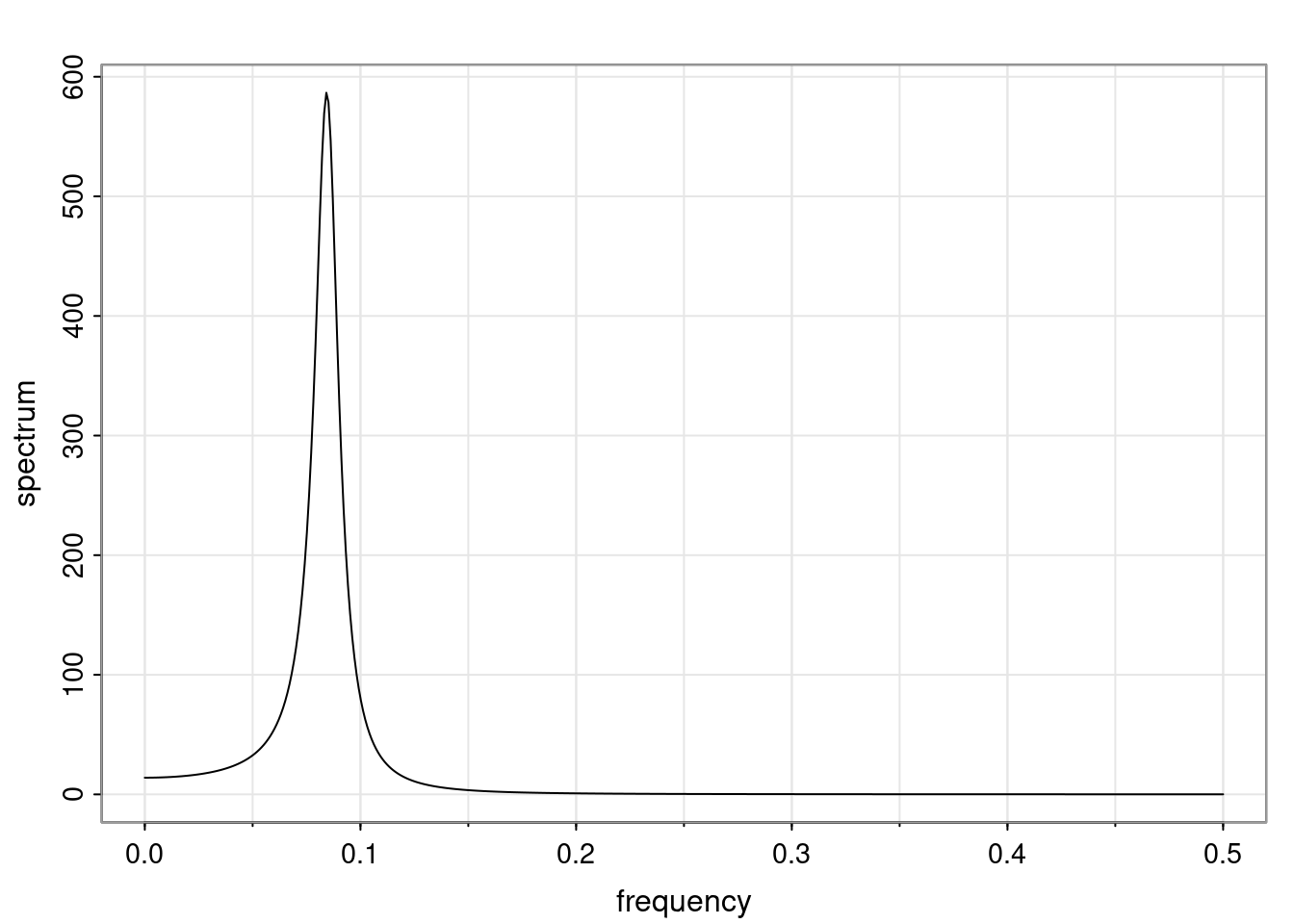
using `arma.spec` from `astsa` package to draw spectral density
plot spectral density of simulated data with posterior sampled ar coefficients and innvovation variance
```{r}
#| label: fig-ar-spectral-density-arma-spec
#| fig-cap: Spectral density of AR(2) process using arma.spec
library("astsa")

par(mfrow = c(1, 1), mar = c(3, 4, 2, 1) )
#result_MLE=arma.spec(ar=phi_MLE, var.noise = s2, log='yes',main = '')
result_MLE=arma.spec(ar=phi_MLE, var.noise = s2, main = '')
freq=result_MLE$freq

spec=matrix(0,nrow=n_sample,ncol=length(freq))

for (i in 1:n_sample){
result=arma.spec(ar=phi_sample[i,], var.noise = v_sample[i],# log='yes',
                 main = '',plot=FALSE)
spec[i,]=result$spec
}
```
```{r}
#| label: fig-ar-spectral-density-plot
#| fig-cap: Spectral density of AR(2) process using arma.spec
plot(2*pi*freq,log(spec[1,]),type='l',ylim=c(-3,12),ylab="log spectra",
     xlab="frequency",col=0)
#for (i in 1:n_sample){
for (i in 1:2){
lines(2*pi*freq,log(spec[i,]),col='darkgray')
}
lines(2*pi*freq,log(result_MLE$spec))
abline(v=2*pi/12,lty=2,col='red')
```
## ARIMA processes :spiral_notepad:
This section introduces the ARMA and ARIMA processes, their definitions, stability, invertibility, and spectral density. It is based on a [handout](handouts/c4-ARIMA.pdf) from the course. Ideally it should be expanded with more details and examples and code for simulating ARMA and ARIMA processes. I'm not sure why Prado didn't go any deeper in the course, but the NDLMs generalize the ARMA and ARIMA processes, so perhaps we will cover them as special cases of the NDLMs in the next lessons.
\index{ARMA process!definition}
::: {.callout-important}
## ARMA Model Definition {.unnumbered}
A time series process is a zero-mean autoregressive moving average process if it is given by
$$
\operatorname{ARMA}(p,q)= \textcolor{red}
{\underbrace{\sum_{i=1}^{p} \phi_i y_{t-i}}_{AR(p)}}
+
\textcolor{blue}
{\underbrace{\sum_{j=1}^{q} \theta_j \varepsilon_{t-j}}_{MA(Q)}}
+ \varepsilon_t
$$ {#eq-arma-definition}
with $\varepsilon_t \sim N(0, v)$.
- For $q = 0$, we get an AR($p$) process.
- For $p = 0$, we get a MA(q) i.e. moving average process of order $q$.
:::
Next we will define the notions of stability and invertibility of an ARMA process.
\index{ARMA process!stability}
::: {.callout-important}
## Stability Definition {.unnumbered}
[stable]{.column-margin}
[An ARMA process is **stable** if the roots of the AR characteristic polynomial]{.mark}
$$
\Phi(u) = 1 - \phi_1 u - \phi_2 u^2 - \ldots - \phi_p u^p
$$
lie outside the unit circle, i.e., for all $u$ such that $\Phi(u) = 0$, $\|u\| > 1$.
Equivalently, this happens when the reciprocal roots of the *AR($p$) polynomial* have moduli smaller than 1.
This condition implies stationarity.
:::
\index{ARMA process!invertibility}
::: {.callout-important}
## Invertible ARMA Definition {.unnumbered}
An ARMA process is **invertible** if the roots of the MA **characteristic polynomial** given by [invertible]{.column-margin}
$$
\Theta(u) = 1 + \theta_1 u + \ldots + \theta_q u^q,
$$ {#eq-arma-ma-poly}
lie outside the unit circle.
:::
Note that $\Phi(B) y_t = \Theta(B) \varepsilon_t$.
- [When an ARMA process is **stable**, it can be written as an infinite order moving average process.]{.mark}
- [When an ARMA process is **invertible**, it can be written as an infinite order autoregressive process.]{.mark}
\index{ARIMA process!definition}
::: {.callout-important}
## ARIMA Processes {.unnumbered}
An autoregressive integrated moving average process with orders $p$, $d$, and $q$ is a process that can be written as
$$
(1 - B)^d y_t = \sum_{i=1}^{p} \phi_i y_{t-i} + \sum_{j=1}^{q} \theta_j \varepsilon_{t-j} + \varepsilon_t,
$$ {#eq-arima-definition}
where $B$ is the backshift operator, $d$ is the order of integration, and $\varepsilon_t \sim N(0, v)$.
in other words, $y_t$ follows an ARIMA(p, d, q) if the $d$ difference of $y_t$ follows an ARMA(p, q).
:::
Estimation in ARIMA processes can be done via *least squares*, *maximum likelihood*, and also *in a Bayesian way*.
We don't discuss Bayesian estimation of ARIMA processes in this course.
### Spectral Density of ARMA Processes
\index{ARMA process!spectral density}
For a given **AR($p$)** process with AR coefficients $\phi_1, \dots, \phi_p$ and variance $v$, we can obtain its **spectral density** as
$$
f(\omega) = \frac{v}{2\pi \|\Phi(e^{-i\omega})\|^2} = \frac{v}{2\pi \|1 - \phi_1 e^{-i\omega} - \ldots - \phi_p e^{-ip\omega}\|^2},
$$ {#eq-ar-spectral-density}
with $\omega$ a frequency in $(0, \pi)$.
The spectral density provides a frequency-domain representation of the process that is appealing because of its interpretability.
For instance, an **AR(2)** process that has one pair of complex-valued reciprocal roots with modulus 0.7 and a period of $\lambda = 12$, will show a mode in the spectral density located at a frequency of $2\pi/12$. If we keep the period of the process at the same value of 12 but increase its modulus to 0.95, the spectral density will continue to show a mode at $2\pi/12$, but the value of $f(2\pi/12)$ will be higher, indicating a more persistent *quasi-periodic* behavior.
Similarly, we can obtain the spectral density of an ARMA process with AR characteristic polynomial $\Phi(u) = 1 - \phi_1 u - \ldots - \phi_p u^p$ and MA characteristic polynomial $\Theta(u) = 1 + \theta_1 u + \ldots + \theta_q u^q$, and variance $v$ as
$$
f(\omega) = \frac{v}{2\pi} \frac{\|\Theta(e^{-i\omega})\|^2}{\|\Phi(e^{-i\omega}) \|^2}.
$$ {#eq-arma-spectral-density}
Note that if we have posterior estimates or posterior samples of the AR/ARMA coefficients and the variance $v$, we can obtain samples from the spectral density of AR/ARMA processes using the equations above.